Note
To run this notebook locally, follow the setup instructions in the GitHub repository.
Use case: ERA5 on a small area#
Earth Data Hub offers an innovative and super-efficient way to access data.
Here we present how to best access the service in the simplest use case.
Setup the environment#
If you haven’t done it already, follow the Getting started notebook to setup your environment and DestinE credentials.
Download 30 years of an ERA5 variable on a small area#
Our use case is to compute various climatological averages of one ERA5 variable over a long period of time, e.g. the surface temperature over 30 years. Note that we will be using the ERA5 single levels dataset that has more than 100 variable and every variable is almost 3TiB in size.
The best practice for downloading data form the Earth Data Hub comprise the following steps:
open the dataset using the code snippet found on the ERA5 dataset page
select the variable
select the area of interest (optionally aligning it on chunk boundaries)
select the time interval of interest
download the data to memory (with
.persist()or.compute())save the data or compute the result in memory
Open the dataset#
The following assumes you set up your EDH API key in your netrc file.
[1]:
import xarray as xr

era5_single_levels_dataset = xr.open_dataset(
    "https://data.earthdatahub.destine.eu/era5/era5-single-levels-atmosphere-v0.zarr",
    storage_options={"client_kwargs": {"trust_env": True}},
    chunks={},
    engine="zarr",
)
era5_single_levels_dataset
[1]:
<xarray.Dataset> Size: 407TB
Dimensions:     (valid_time: 760440, latitude: 721, longitude: 1440)
Coordinates:
  * valid_time  (valid_time) datetime64[ns] 6MB 1940-01-01 ... 2026-09-30T23:...
  * latitude    (latitude) float64 6kB 90.0 89.75 89.5 ... -89.5 -89.75 -90.0
  * longitude   (longitude) float64 12kB 0.0 0.25 0.5 0.75 ... 359.2 359.5 359.8
Data variables: (12/129)
    alnid       (valid_time, latitude, longitude) float32 3TB dask.array<chunksize=(1080, 60, 60), meta=np.ndarray>
    alnip       (valid_time, latitude, longitude) float32 3TB dask.array<chunksize=(1080, 60, 60), meta=np.ndarray>
    aluvd       (valid_time, latitude, longitude) float32 3TB dask.array<chunksize=(1080, 60, 60), meta=np.ndarray>
    aluvp       (valid_time, latitude, longitude) float32 3TB dask.array<chunksize=(1080, 60, 60), meta=np.ndarray>
    anor        (valid_time, latitude, longitude) float32 3TB dask.array<chunksize=(1080, 60, 60), meta=np.ndarray>
    asn         (valid_time, latitude, longitude) float32 3TB dask.array<chunksize=(1080, 60, 60), meta=np.ndarray>
    ...          ...
    viiwn       (valid_time, latitude, longitude) float32 3TB dask.array<chunksize=(1080, 60, 60), meta=np.ndarray>
    vilwd       (valid_time, latitude, longitude) float32 3TB dask.array<chunksize=(1080, 60, 60), meta=np.ndarray>
    vilwe       (valid_time, latitude, longitude) float32 3TB dask.array<chunksize=(1080, 60, 60), meta=np.ndarray>
    vilwn       (valid_time, latitude, longitude) float32 3TB dask.array<chunksize=(1080, 60, 60), meta=np.ndarray>
    z           (valid_time, latitude, longitude) float32 3TB dask.array<chunksize=(1080, 60, 60), meta=np.ndarray>
    zust        (valid_time, latitude, longitude) float32 3TB dask.array<chunksize=(1080, 60, 60), meta=np.ndarray>
Attributes:
    GRIB_edition:            1
    GRIB_centre:             ecmf
    GRIB_centreDescription:  European Centre for Medium-Range Weather Forecasts
    GRIB_subCentre:          0
    Conventions:             CF-1.7
    institution:             European Centre for Medium-Range Weather Forecasts
history: 2026-08-19T13:34 GRIB to CDM+CF via cfgrib-0.9.1...- valid_time: 760440
- latitude: 721
- longitude: 1440
- valid_time(valid_time)datetime64[ns]1940-01-01 ... 2026-09-30T23:00:00
array(['1940-01-01T00:00:00.000000000', '1940-01-01T01:00:00.000000000', '1940-01-01T02:00:00.000000000', ..., '2026-09-30T21:00:00.000000000', '2026-09-30T22:00:00.000000000', '2026-09-30T23:00:00.000000000'], shape=(760440,), dtype='datetime64[ns]') - latitude(latitude)float6490.0 89.75 89.5 ... -89.75 -90.0
- units :
- degrees_north
- standard_name :
- latitude
- long_name :
- latitude
- stored_direction :
- decreasing
array([ 90. , 89.75, 89.5 , ..., -89.5 , -89.75, -90. ], shape=(721,))
- longitude(longitude)float640.0 0.25 0.5 ... 359.2 359.5 359.8
- units :
- degrees_east
- standard_name :
- longitude
- long_name :
- longitude
array([0.0000e+00, 2.5000e-01, 5.0000e-01, ..., 3.5925e+02, 3.5950e+02,
       3.5975e+02], shape=(1440,))
- alnid(valid_time, latitude, longitude)float32dask.array<chunksize=(1080, 60, 60), meta=np.ndarray>
- GRIB_paramId :
- 18
- GRIB_dataType :
- an
- GRIB_numberOfPoints :
- 1038240
- GRIB_typeOfLevel :
- surface
- GRIB_stepUnits :
- 1
- GRIB_stepType :
- instant
- GRIB_gridType :
- regular_ll
- GRIB_uvRelativeToGrid :
- 0
- GRIB_NV :
- 0
- GRIB_Nx :
- 1440
- GRIB_Ny :
- 721
- GRIB_cfName :
- unknown
- GRIB_cfVarName :
- alnid
- GRIB_gridDefinitionDescription :
- Latitude/Longitude Grid
- GRIB_iDirectionIncrementInDegrees :
- 0.25
- GRIB_iScansNegatively :
- 0
- GRIB_jDirectionIncrementInDegrees :
- 0.25
- GRIB_jPointsAreConsecutive :
- 0
- GRIB_jScansPositively :
- 0
- GRIB_latitudeOfFirstGridPointInDegrees :
- 90.0
- GRIB_latitudeOfLastGridPointInDegrees :
- -90.0
- GRIB_longitudeOfFirstGridPointInDegrees :
- 0.0
- GRIB_longitudeOfLastGridPointInDegrees :
- 359.75
- GRIB_missingValue :
- 3.4028234663852886e+38
- GRIB_name :
- Near IR albedo for diffuse radiation (climatological)
- GRIB_shortName :
- alnid
- GRIB_totalNumber :
- 0
- GRIB_units :
- (0 - 1)
- long_name :
- Near IR albedo for diffuse radiation (climatological)
- units :
- (0 - 1)
- standard_name :
- unknown
- last_ingested_valid_time_index :
- 760439
Array Chunk Bytes 2.87 TiB 14.83 MiB Shape (760440, 721, 1440) (1080, 60, 60) Dask graph 219960 chunks in 2 graph layers Data type float32 numpy.ndarray - alnip(valid_time, latitude, longitude)float32dask.array<chunksize=(1080, 60, 60), meta=np.ndarray>
- GRIB_paramId :
- 17
- GRIB_dataType :
- an
- GRIB_numberOfPoints :
- 1038240
- GRIB_typeOfLevel :
- surface
- GRIB_stepUnits :
- 1
- GRIB_stepType :
- instant
- GRIB_gridType :
- regular_ll
- GRIB_uvRelativeToGrid :
- 0
- GRIB_NV :
- 0
- GRIB_Nx :
- 1440
- GRIB_Ny :
- 721
- GRIB_cfName :
- unknown
- GRIB_cfVarName :
- alnip
- GRIB_gridDefinitionDescription :
- Latitude/Longitude Grid
- GRIB_iDirectionIncrementInDegrees :
- 0.25
- GRIB_iScansNegatively :
- 0
- GRIB_jDirectionIncrementInDegrees :
- 0.25
- GRIB_jPointsAreConsecutive :
- 0
- GRIB_jScansPositively :
- 0
- GRIB_latitudeOfFirstGridPointInDegrees :
- 90.0
- GRIB_latitudeOfLastGridPointInDegrees :
- -90.0
- GRIB_longitudeOfFirstGridPointInDegrees :
- 0.0
- GRIB_longitudeOfLastGridPointInDegrees :
- 359.75
- GRIB_missingValue :
- 3.4028234663852886e+38
- GRIB_name :
- Near IR albedo for direct radiation (climatological)
- GRIB_shortName :
- alnip
- GRIB_totalNumber :
- 0
- GRIB_units :
- (0 - 1)
- long_name :
- Near IR albedo for direct radiation (climatological)
- units :
- (0 - 1)
- standard_name :
- unknown
- last_ingested_valid_time_index :
- 760439
Array Chunk Bytes 2.87 TiB 14.83 MiB Shape (760440, 721, 1440) (1080, 60, 60) Dask graph 219960 chunks in 2 graph layers Data type float32 numpy.ndarray - aluvd(valid_time, latitude, longitude)float32dask.array<chunksize=(1080, 60, 60), meta=np.ndarray>
- GRIB_paramId :
- 16
- GRIB_dataType :
- an
- GRIB_numberOfPoints :
- 1038240
- GRIB_typeOfLevel :
- surface
- GRIB_stepUnits :
- 1
- GRIB_stepType :
- instant
- GRIB_gridType :
- regular_ll
- GRIB_uvRelativeToGrid :
- 0
- GRIB_NV :
- 0
- GRIB_Nx :
- 1440
- GRIB_Ny :
- 721
- GRIB_cfName :
- unknown
- GRIB_cfVarName :
- aluvd
- GRIB_gridDefinitionDescription :
- Latitude/Longitude Grid
- GRIB_iDirectionIncrementInDegrees :
- 0.25
- GRIB_iScansNegatively :
- 0
- GRIB_jDirectionIncrementInDegrees :
- 0.25
- GRIB_jPointsAreConsecutive :
- 0
- GRIB_jScansPositively :
- 0
- GRIB_latitudeOfFirstGridPointInDegrees :
- 90.0
- GRIB_latitudeOfLastGridPointInDegrees :
- -90.0
- GRIB_longitudeOfFirstGridPointInDegrees :
- 0.0
- GRIB_longitudeOfLastGridPointInDegrees :
- 359.75
- GRIB_missingValue :
- 3.4028234663852886e+38
- GRIB_name :
- UV visible albedo for diffuse radiation (climatological)
- GRIB_shortName :
- aluvd
- GRIB_totalNumber :
- 0
- GRIB_units :
- (0 - 1)
- long_name :
- UV visible albedo for diffuse radiation (climatological)
- units :
- (0 - 1)
- standard_name :
- unknown
- last_ingested_valid_time_index :
- 760439
Array Chunk Bytes 2.87 TiB 14.83 MiB Shape (760440, 721, 1440) (1080, 60, 60) Dask graph 219960 chunks in 2 graph layers Data type float32 numpy.ndarray - aluvp(valid_time, latitude, longitude)float32dask.array<chunksize=(1080, 60, 60), meta=np.ndarray>
- GRIB_paramId :
- 15
- GRIB_dataType :
- an
- GRIB_numberOfPoints :
- 1038240
- GRIB_typeOfLevel :
- surface
- GRIB_stepUnits :
- 1
- GRIB_stepType :
- instant
- GRIB_gridType :
- regular_ll
- GRIB_uvRelativeToGrid :
- 0
- GRIB_NV :
- 0
- GRIB_Nx :
- 1440
- GRIB_Ny :
- 721
- GRIB_cfName :
- unknown
- GRIB_cfVarName :
- aluvp
- GRIB_gridDefinitionDescription :
- Latitude/Longitude Grid
- GRIB_iDirectionIncrementInDegrees :
- 0.25
- GRIB_iScansNegatively :
- 0
- GRIB_jDirectionIncrementInDegrees :
- 0.25
- GRIB_jPointsAreConsecutive :
- 0
- GRIB_jScansPositively :
- 0
- GRIB_latitudeOfFirstGridPointInDegrees :
- 90.0
- GRIB_latitudeOfLastGridPointInDegrees :
- -90.0
- GRIB_longitudeOfFirstGridPointInDegrees :
- 0.0
- GRIB_longitudeOfLastGridPointInDegrees :
- 359.75
- GRIB_missingValue :
- 3.4028234663852886e+38
- GRIB_name :
- UV visible albedo for direct radiation (climatological)
- GRIB_shortName :
- aluvp
- GRIB_totalNumber :
- 0
- GRIB_units :
- (0 - 1)
- long_name :
- UV visible albedo for direct radiation (climatological)
- units :
- (0 - 1)
- standard_name :
- unknown
- last_ingested_valid_time_index :
- 760439
Array Chunk Bytes 2.87 TiB 14.83 MiB Shape (760440, 721, 1440) (1080, 60, 60) Dask graph 219960 chunks in 2 graph layers Data type float32 numpy.ndarray - anor(valid_time, latitude, longitude)float32dask.array<chunksize=(1080, 60, 60), meta=np.ndarray>
- GRIB_paramId :
- 162
- GRIB_dataType :
- an
- GRIB_numberOfPoints :
- 1038240
- GRIB_typeOfLevel :
- surface
- GRIB_stepUnits :
- 1
- GRIB_stepType :
- instant
- GRIB_gridType :
- regular_ll
- GRIB_uvRelativeToGrid :
- 0
- GRIB_NV :
- 0
- GRIB_Nx :
- 1440
- GRIB_Ny :
- 721
- GRIB_cfName :
- unknown
- GRIB_cfVarName :
- anor
- GRIB_gridDefinitionDescription :
- Latitude/Longitude Grid
- GRIB_iDirectionIncrementInDegrees :
- 0.25
- GRIB_iScansNegatively :
- 0
- GRIB_jDirectionIncrementInDegrees :
- 0.25
- GRIB_jPointsAreConsecutive :
- 0
- GRIB_jScansPositively :
- 0
- GRIB_latitudeOfFirstGridPointInDegrees :
- 90.0
- GRIB_latitudeOfLastGridPointInDegrees :
- -90.0
- GRIB_longitudeOfFirstGridPointInDegrees :
- 0.0
- GRIB_longitudeOfLastGridPointInDegrees :
- 359.75
- GRIB_missingValue :
- 3.4028234663852886e+38
- GRIB_name :
- Angle of sub-gridscale orography
- GRIB_shortName :
- anor
- GRIB_totalNumber :
- 0
- GRIB_units :
- radians
- long_name :
- Angle of sub-gridscale orography
- units :
- radians
- standard_name :
- unknown
- last_ingested_valid_time_index :
- 760439
Array Chunk Bytes 2.87 TiB 14.83 MiB Shape (760440, 721, 1440) (1080, 60, 60) Dask graph 219960 chunks in 2 graph layers Data type float32 numpy.ndarray - asn(valid_time, latitude, longitude)float32dask.array<chunksize=(1080, 60, 60), meta=np.ndarray>
- GRIB_paramId :
- 32
- GRIB_dataType :
- an
- GRIB_numberOfPoints :
- 1038240
- GRIB_typeOfLevel :
- surface
- GRIB_stepUnits :
- 1
- GRIB_stepType :
- instant
- GRIB_gridType :
- regular_ll
- GRIB_uvRelativeToGrid :
- 0
- GRIB_NV :
- 0
- GRIB_Nx :
- 1440
- GRIB_Ny :
- 721
- GRIB_cfName :
- unknown
- GRIB_cfVarName :
- asn
- GRIB_gridDefinitionDescription :
- Latitude/Longitude Grid
- GRIB_iDirectionIncrementInDegrees :
- 0.25
- GRIB_iScansNegatively :
- 0
- GRIB_jDirectionIncrementInDegrees :
- 0.25
- GRIB_jPointsAreConsecutive :
- 0
- GRIB_jScansPositively :
- 0
- GRIB_latitudeOfFirstGridPointInDegrees :
- 90.0
- GRIB_latitudeOfLastGridPointInDegrees :
- -90.0
- GRIB_longitudeOfFirstGridPointInDegrees :
- 0.0
- GRIB_longitudeOfLastGridPointInDegrees :
- 359.75
- GRIB_missingValue :
- 3.4028234663852886e+38
- GRIB_name :
- Snow albedo
- GRIB_shortName :
- asn
- GRIB_totalNumber :
- 0
- GRIB_units :
- (0 - 1)
- long_name :
- Snow albedo
- units :
- (0 - 1)
- standard_name :
- unknown
- last_ingested_valid_time_index :
- 760439
Array Chunk Bytes 2.87 TiB 14.83 MiB Shape (760440, 721, 1440) (1080, 60, 60) Dask graph 219960 chunks in 2 graph layers Data type float32 numpy.ndarray - bld(valid_time, latitude, longitude)float32dask.array<chunksize=(1080, 60, 60), meta=np.ndarray>
- GRIB_paramId :
- 145
- GRIB_dataType :
- fc
- GRIB_numberOfPoints :
- 1038240
- GRIB_typeOfLevel :
- surface
- GRIB_stepUnits :
- 1
- GRIB_stepType :
- accum
- GRIB_gridType :
- regular_ll
- GRIB_uvRelativeToGrid :
- 0
- GRIB_NV :
- 0
- GRIB_Nx :
- 1440
- GRIB_Ny :
- 721
- GRIB_cfName :
- kinetic_energy_dissipation_in_atmosphere_boundary_layer
- GRIB_cfVarName :
- bld
- GRIB_gridDefinitionDescription :
- Latitude/Longitude Grid
- GRIB_iDirectionIncrementInDegrees :
- 0.25
- GRIB_iScansNegatively :
- 0
- GRIB_jDirectionIncrementInDegrees :
- 0.25
- GRIB_jPointsAreConsecutive :
- 0
- GRIB_jScansPositively :
- 0
- GRIB_latitudeOfFirstGridPointInDegrees :
- 90.0
- GRIB_latitudeOfLastGridPointInDegrees :
- -90.0
- GRIB_longitudeOfFirstGridPointInDegrees :
- 0.0
- GRIB_longitudeOfLastGridPointInDegrees :
- 359.75
- GRIB_missingValue :
- 3.4028234663852886e+38
- GRIB_name :
- Time-integrated boundary layer dissipation
- GRIB_shortName :
- bld
- GRIB_totalNumber :
- 0
- GRIB_units :
- J m**-2
- long_name :
- Time-integrated boundary layer dissipation
- units :
- J m**-2
- standard_name :
- kinetic_energy_dissipation_in_atmosphere_boundary_layer
- last_ingested_valid_time_index :
- 760439
Array Chunk Bytes 2.87 TiB 14.83 MiB Shape (760440, 721, 1440) (1080, 60, 60) Dask graph 219960 chunks in 2 graph layers Data type float32 numpy.ndarray - blh(valid_time, latitude, longitude)float32dask.array<chunksize=(1080, 60, 60), meta=np.ndarray>
- GRIB_paramId :
- 159
- GRIB_dataType :
- an
- GRIB_numberOfPoints :
- 1038240
- GRIB_typeOfLevel :
- surface
- GRIB_stepUnits :
- 1
- GRIB_stepType :
- instant
- GRIB_gridType :
- regular_ll
- GRIB_uvRelativeToGrid :
- 0
- GRIB_NV :
- 0
- GRIB_Nx :
- 1440
- GRIB_Ny :
- 721
- GRIB_cfName :
- unknown
- GRIB_cfVarName :
- blh
- GRIB_gridDefinitionDescription :
- Latitude/Longitude Grid
- GRIB_iDirectionIncrementInDegrees :
- 0.25
- GRIB_iScansNegatively :
- 0
- GRIB_jDirectionIncrementInDegrees :
- 0.25
- GRIB_jPointsAreConsecutive :
- 0
- GRIB_jScansPositively :
- 0
- GRIB_latitudeOfFirstGridPointInDegrees :
- 90.0
- GRIB_latitudeOfLastGridPointInDegrees :
- -90.0
- GRIB_longitudeOfFirstGridPointInDegrees :
- 0.0
- GRIB_longitudeOfLastGridPointInDegrees :
- 359.75
- GRIB_missingValue :
- 3.4028234663852886e+38
- GRIB_name :
- Boundary layer height
- GRIB_shortName :
- blh
- GRIB_totalNumber :
- 0
- GRIB_units :
- m
- long_name :
- Boundary layer height
- units :
- m
- standard_name :
- unknown
- last_ingested_valid_time_index :
- 760439
Array Chunk Bytes 2.87 TiB 14.83 MiB Shape (760440, 721, 1440) (1080, 60, 60) Dask graph 219960 chunks in 2 graph layers Data type float32 numpy.ndarray - cape(valid_time, latitude, longitude)float32dask.array<chunksize=(1080, 60, 60), meta=np.ndarray>
- GRIB_paramId :
- 59
- GRIB_dataType :
- an
- GRIB_numberOfPoints :
- 1038240
- GRIB_typeOfLevel :
- surface
- GRIB_stepUnits :
- 1
- GRIB_stepType :
- instant
- GRIB_gridType :
- regular_ll
- GRIB_uvRelativeToGrid :
- 0
- GRIB_NV :
- 0
- GRIB_Nx :
- 1440
- GRIB_Ny :
- 721
- GRIB_cfName :
- unknown
- GRIB_cfVarName :
- cape
- GRIB_gridDefinitionDescription :
- Latitude/Longitude Grid
- GRIB_iDirectionIncrementInDegrees :
- 0.25
- GRIB_iScansNegatively :
- 0
- GRIB_jDirectionIncrementInDegrees :
- 0.25
- GRIB_jPointsAreConsecutive :
- 0
- GRIB_jScansPositively :
- 0
- GRIB_latitudeOfFirstGridPointInDegrees :
- 90.0
- GRIB_latitudeOfLastGridPointInDegrees :
- -90.0
- GRIB_longitudeOfFirstGridPointInDegrees :
- 0.0
- GRIB_longitudeOfLastGridPointInDegrees :
- 359.75
- GRIB_missingValue :
- 3.4028234663852886e+38
- GRIB_name :
- Convective available potential energy
- GRIB_shortName :
- cape
- GRIB_totalNumber :
- 0
- GRIB_units :
- J kg**-1
- long_name :
- Convective available potential energy
- units :
- J kg**-1
- standard_name :
- unknown
- last_ingested_valid_time_index :
- 760439
Array Chunk Bytes 2.87 TiB 14.83 MiB Shape (760440, 721, 1440) (1080, 60, 60) Dask graph 219960 chunks in 2 graph layers Data type float32 numpy.ndarray - cdir(valid_time, latitude, longitude)float32dask.array<chunksize=(1080, 60, 60), meta=np.ndarray>
- GRIB_paramId :
- 228022
- GRIB_dataType :
- fc
- GRIB_numberOfPoints :
- 1038240
- GRIB_typeOfLevel :
- surface
- GRIB_stepUnits :
- 1
- GRIB_stepType :
- accum
- GRIB_gridType :
- regular_ll
- GRIB_uvRelativeToGrid :
- 0
- GRIB_NV :
- 0
- GRIB_Nx :
- 1440
- GRIB_Ny :
- 721
- GRIB_cfName :
- unknown
- GRIB_cfVarName :
- cdir
- GRIB_gridDefinitionDescription :
- Latitude/Longitude Grid
- GRIB_iDirectionIncrementInDegrees :
- 0.25
- GRIB_iScansNegatively :
- 0
- GRIB_jDirectionIncrementInDegrees :
- 0.25
- GRIB_jPointsAreConsecutive :
- 0
- GRIB_jScansPositively :
- 0
- GRIB_latitudeOfFirstGridPointInDegrees :
- 90.0
- GRIB_latitudeOfLastGridPointInDegrees :
- -90.0
- GRIB_longitudeOfFirstGridPointInDegrees :
- 0.0
- GRIB_longitudeOfLastGridPointInDegrees :
- 359.75
- GRIB_missingValue :
- 3.4028234663852886e+38
- GRIB_name :
- Surface direct short-wave radiation, clear sky
- GRIB_shortName :
- cdir
- GRIB_totalNumber :
- 0
- GRIB_units :
- J m**-2
- long_name :
- Surface direct short-wave radiation, clear sky
- units :
- J m**-2
- standard_name :
- unknown
- last_ingested_valid_time_index :
- 760439
Array Chunk Bytes 2.87 TiB 14.83 MiB Shape (760440, 721, 1440) (1080, 60, 60) Dask graph 219960 chunks in 2 graph layers Data type float32 numpy.ndarray - chnk(valid_time, latitude, longitude)float32dask.array<chunksize=(1080, 60, 60), meta=np.ndarray>
- GRIB_paramId :
- 148
- GRIB_dataType :
- an
- GRIB_numberOfPoints :
- 1038240
- GRIB_typeOfLevel :
- surface
- GRIB_stepUnits :
- 1
- GRIB_stepType :
- instant
- GRIB_gridType :
- regular_ll
- GRIB_uvRelativeToGrid :
- 0
- GRIB_NV :
- 0
- GRIB_Nx :
- 1440
- GRIB_Ny :
- 721
- GRIB_cfName :
- unknown
- GRIB_cfVarName :
- chnk
- GRIB_gridDefinitionDescription :
- Latitude/Longitude Grid
- GRIB_iDirectionIncrementInDegrees :
- 0.25
- GRIB_iScansNegatively :
- 0
- GRIB_jDirectionIncrementInDegrees :
- 0.25
- GRIB_jPointsAreConsecutive :
- 0
- GRIB_jScansPositively :
- 0
- GRIB_latitudeOfFirstGridPointInDegrees :
- 90.0
- GRIB_latitudeOfLastGridPointInDegrees :
- -90.0
- GRIB_longitudeOfFirstGridPointInDegrees :
- 0.0
- GRIB_longitudeOfLastGridPointInDegrees :
- 359.75
- GRIB_missingValue :
- 3.4028234663852886e+38
- GRIB_name :
- Charnock
- GRIB_shortName :
- chnk
- GRIB_totalNumber :
- 0
- GRIB_units :
- Numeric
- long_name :
- Charnock
- units :
- Numeric
- standard_name :
- unknown
- last_ingested_valid_time_index :
- 760439
Array Chunk Bytes 2.87 TiB 14.83 MiB Shape (760440, 721, 1440) (1080, 60, 60) Dask graph 219960 chunks in 2 graph layers Data type float32 numpy.ndarray - cin(valid_time, latitude, longitude)float32dask.array<chunksize=(1080, 60, 60), meta=np.ndarray>
- GRIB_paramId :
- 228001
- GRIB_dataType :
- fc
- GRIB_numberOfPoints :
- 1038240
- GRIB_typeOfLevel :
- surface
- GRIB_stepUnits :
- 1
- GRIB_stepType :
- instant
- GRIB_gridType :
- regular_ll
- GRIB_uvRelativeToGrid :
- 0
- GRIB_NV :
- 0
- GRIB_Nx :
- 1440
- GRIB_Ny :
- 721
- GRIB_cfName :
- unknown
- GRIB_cfVarName :
- cin
- GRIB_gridDefinitionDescription :
- Latitude/Longitude Grid
- GRIB_iDirectionIncrementInDegrees :
- 0.25
- GRIB_iScansNegatively :
- 0
- GRIB_jDirectionIncrementInDegrees :
- 0.25
- GRIB_jPointsAreConsecutive :
- 0
- GRIB_jScansPositively :
- 0
- GRIB_latitudeOfFirstGridPointInDegrees :
- 90.0
- GRIB_latitudeOfLastGridPointInDegrees :
- -90.0
- GRIB_longitudeOfFirstGridPointInDegrees :
- 0.0
- GRIB_longitudeOfLastGridPointInDegrees :
- 359.75
- GRIB_missingValue :
- 3.4028234663852886e+38
- GRIB_name :
- Convective inhibition
- GRIB_shortName :
- cin
- GRIB_totalNumber :
- 0
- GRIB_units :
- J kg**-1
- long_name :
- Convective inhibition
- units :
- J kg**-1
- standard_name :
- unknown
- last_ingested_valid_time_index :
- 760439
Array Chunk Bytes 2.87 TiB 14.83 MiB Shape (760440, 721, 1440) (1080, 60, 60) Dask graph 219960 chunks in 2 graph layers Data type float32 numpy.ndarray - cl(valid_time, latitude, longitude)float32dask.array<chunksize=(1080, 60, 60), meta=np.ndarray>
- GRIB_paramId :
- 26
- GRIB_dataType :
- an
- GRIB_numberOfPoints :
- 1038240
- GRIB_typeOfLevel :
- surface
- GRIB_stepUnits :
- 1
- GRIB_stepType :
- instant
- GRIB_gridType :
- regular_ll
- GRIB_uvRelativeToGrid :
- 0
- GRIB_NV :
- 0
- GRIB_Nx :
- 1440
- GRIB_Ny :
- 721
- GRIB_cfName :
- unknown
- GRIB_cfVarName :
- cl
- GRIB_gridDefinitionDescription :
- Latitude/Longitude Grid
- GRIB_iDirectionIncrementInDegrees :
- 0.25
- GRIB_iScansNegatively :
- 0
- GRIB_jDirectionIncrementInDegrees :
- 0.25
- GRIB_jPointsAreConsecutive :
- 0
- GRIB_jScansPositively :
- 0
- GRIB_latitudeOfFirstGridPointInDegrees :
- 90.0
- GRIB_latitudeOfLastGridPointInDegrees :
- -90.0
- GRIB_longitudeOfFirstGridPointInDegrees :
- 0.0
- GRIB_longitudeOfLastGridPointInDegrees :
- 359.75
- GRIB_missingValue :
- 3.4028234663852886e+38
- GRIB_name :
- Lake cover
- GRIB_shortName :
- cl
- GRIB_totalNumber :
- 0
- GRIB_units :
- (0 - 1)
- long_name :
- Lake cover
- units :
- (0 - 1)
- standard_name :
- unknown
- last_ingested_valid_time_index :
- 760439
Array Chunk Bytes 2.87 TiB 14.83 MiB Shape (760440, 721, 1440) (1080, 60, 60) Dask graph 219960 chunks in 2 graph layers Data type float32 numpy.ndarray - cp(valid_time, latitude, longitude)float32dask.array<chunksize=(1080, 60, 60), meta=np.ndarray>
- GRIB_paramId :
- 143
- GRIB_dataType :
- fc
- GRIB_numberOfPoints :
- 1038240
- GRIB_typeOfLevel :
- surface
- GRIB_stepUnits :
- 1
- GRIB_stepType :
- accum
- GRIB_gridType :
- regular_ll
- GRIB_uvRelativeToGrid :
- 0
- GRIB_NV :
- 0
- GRIB_Nx :
- 1440
- GRIB_Ny :
- 721
- GRIB_cfName :
- lwe_thickness_of_convective_precipitation_amount
- GRIB_cfVarName :
- cp
- GRIB_gridDefinitionDescription :
- Latitude/Longitude Grid
- GRIB_iDirectionIncrementInDegrees :
- 0.25
- GRIB_iScansNegatively :
- 0
- GRIB_jDirectionIncrementInDegrees :
- 0.25
- GRIB_jPointsAreConsecutive :
- 0
- GRIB_jScansPositively :
- 0
- GRIB_latitudeOfFirstGridPointInDegrees :
- 90.0
- GRIB_latitudeOfLastGridPointInDegrees :
- -90.0
- GRIB_longitudeOfFirstGridPointInDegrees :
- 0.0
- GRIB_longitudeOfLastGridPointInDegrees :
- 359.75
- GRIB_missingValue :
- 3.4028234663852886e+38
- GRIB_name :
- Convective precipitation
- GRIB_shortName :
- cp
- GRIB_totalNumber :
- 0
- GRIB_units :
- m
- long_name :
- Convective precipitation
- units :
- m
- standard_name :
- lwe_thickness_of_convective_precipitation_amount
- last_ingested_valid_time_index :
- 760439
Array Chunk Bytes 2.87 TiB 14.83 MiB Shape (760440, 721, 1440) (1080, 60, 60) Dask graph 219960 chunks in 2 graph layers Data type float32 numpy.ndarray - crr(valid_time, latitude, longitude)float32dask.array<chunksize=(1080, 60, 60), meta=np.ndarray>
- GRIB_paramId :
- 228218
- GRIB_dataType :
- fc
- GRIB_numberOfPoints :
- 1038240
- GRIB_typeOfLevel :
- surface
- GRIB_stepUnits :
- 1
- GRIB_stepType :
- instant
- GRIB_gridType :
- regular_ll
- GRIB_uvRelativeToGrid :
- 0
- GRIB_NV :
- 0
- GRIB_Nx :
- 1440
- GRIB_Ny :
- 721
- GRIB_cfName :
- unknown
- GRIB_cfVarName :
- crr
- GRIB_gridDefinitionDescription :
- Latitude/Longitude Grid
- GRIB_iDirectionIncrementInDegrees :
- 0.25
- GRIB_iScansNegatively :
- 0
- GRIB_jDirectionIncrementInDegrees :
- 0.25
- GRIB_jPointsAreConsecutive :
- 0
- GRIB_jScansPositively :
- 0
- GRIB_latitudeOfFirstGridPointInDegrees :
- 90.0
- GRIB_latitudeOfLastGridPointInDegrees :
- -90.0
- GRIB_longitudeOfFirstGridPointInDegrees :
- 0.0
- GRIB_longitudeOfLastGridPointInDegrees :
- 359.75
- GRIB_missingValue :
- 3.4028234663852886e+38
- GRIB_name :
- Convective rain rate
- GRIB_shortName :
- crr
- GRIB_totalNumber :
- 0
- GRIB_units :
- kg m**-2 s**-1
- long_name :
- Convective rain rate
- units :
- kg m**-2 s**-1
- standard_name :
- unknown
- last_ingested_valid_time_index :
- 760439
Array Chunk Bytes 2.87 TiB 14.83 MiB Shape (760440, 721, 1440) (1080, 60, 60) Dask graph 219960 chunks in 2 graph layers Data type float32 numpy.ndarray - csf(valid_time, latitude, longitude)float32dask.array<chunksize=(1080, 60, 60), meta=np.ndarray>
- GRIB_paramId :
- 239
- GRIB_dataType :
- fc
- GRIB_numberOfPoints :
- 1038240
- GRIB_typeOfLevel :
- surface
- GRIB_stepUnits :
- 1
- GRIB_stepType :
- accum
- GRIB_gridType :
- regular_ll
- GRIB_uvRelativeToGrid :
- 0
- GRIB_NV :
- 0
- GRIB_Nx :
- 1440
- GRIB_Ny :
- 721
- GRIB_cfName :
- unknown
- GRIB_cfVarName :
- csf
- GRIB_gridDefinitionDescription :
- Latitude/Longitude Grid
- GRIB_iDirectionIncrementInDegrees :
- 0.25
- GRIB_iScansNegatively :
- 0
- GRIB_jDirectionIncrementInDegrees :
- 0.25
- GRIB_jPointsAreConsecutive :
- 0
- GRIB_jScansPositively :
- 0
- GRIB_latitudeOfFirstGridPointInDegrees :
- 90.0
- GRIB_latitudeOfLastGridPointInDegrees :
- -90.0
- GRIB_longitudeOfFirstGridPointInDegrees :
- 0.0
- GRIB_longitudeOfLastGridPointInDegrees :
- 359.75
- GRIB_missingValue :
- 3.4028234663852886e+38
- GRIB_name :
- Convective snowfall
- GRIB_shortName :
- csf
- GRIB_totalNumber :
- 0
- GRIB_units :
- m of water equivalent
- long_name :
- Convective snowfall
- units :
- m of water equivalent
- standard_name :
- unknown
- last_ingested_valid_time_index :
- 760439
Array Chunk Bytes 2.87 TiB 14.83 MiB Shape (760440, 721, 1440) (1080, 60, 60) Dask graph 219960 chunks in 2 graph layers Data type float32 numpy.ndarray - csfr(valid_time, latitude, longitude)float32dask.array<chunksize=(1080, 60, 60), meta=np.ndarray>
- GRIB_paramId :
- 228220
- GRIB_dataType :
- fc
- GRIB_numberOfPoints :
- 1038240
- GRIB_typeOfLevel :
- surface
- GRIB_stepUnits :
- 1
- GRIB_stepType :
- instant
- GRIB_gridType :
- regular_ll
- GRIB_uvRelativeToGrid :
- 0
- GRIB_NV :
- 0
- GRIB_Nx :
- 1440
- GRIB_Ny :
- 721
- GRIB_cfName :
- unknown
- GRIB_cfVarName :
- csfr
- GRIB_gridDefinitionDescription :
- Latitude/Longitude Grid
- GRIB_iDirectionIncrementInDegrees :
- 0.25
- GRIB_iScansNegatively :
- 0
- GRIB_jDirectionIncrementInDegrees :
- 0.25
- GRIB_jPointsAreConsecutive :
- 0
- GRIB_jScansPositively :
- 0
- GRIB_latitudeOfFirstGridPointInDegrees :
- 90.0
- GRIB_latitudeOfLastGridPointInDegrees :
- -90.0
- GRIB_longitudeOfFirstGridPointInDegrees :
- 0.0
- GRIB_longitudeOfLastGridPointInDegrees :
- 359.75
- GRIB_missingValue :
- 3.4028234663852886e+38
- GRIB_name :
- Convective snowfall rate water equivalent
- GRIB_shortName :
- csfr
- GRIB_totalNumber :
- 0
- GRIB_units :
- kg m**-2 s**-1
- long_name :
- Convective snowfall rate water equivalent
- units :
- kg m**-2 s**-1
- standard_name :
- unknown
- last_ingested_valid_time_index :
- 760439
Array Chunk Bytes 2.87 TiB 14.83 MiB Shape (760440, 721, 1440) (1080, 60, 60) Dask graph 219960 chunks in 2 graph layers Data type float32 numpy.ndarray - cvh(valid_time, latitude, longitude)float32dask.array<chunksize=(1080, 60, 60), meta=np.ndarray>
- GRIB_paramId :
- 28
- GRIB_dataType :
- an
- GRIB_numberOfPoints :
- 1038240
- GRIB_typeOfLevel :
- surface
- GRIB_stepUnits :
- 1
- GRIB_stepType :
- instant
- GRIB_gridType :
- regular_ll
- GRIB_uvRelativeToGrid :
- 0
- GRIB_NV :
- 0
- GRIB_Nx :
- 1440
- GRIB_Ny :
- 721
- GRIB_cfName :
- unknown
- GRIB_cfVarName :
- cvh
- GRIB_gridDefinitionDescription :
- Latitude/Longitude Grid
- GRIB_iDirectionIncrementInDegrees :
- 0.25
- GRIB_iScansNegatively :
- 0
- GRIB_jDirectionIncrementInDegrees :
- 0.25
- GRIB_jPointsAreConsecutive :
- 0
- GRIB_jScansPositively :
- 0
- GRIB_latitudeOfFirstGridPointInDegrees :
- 90.0
- GRIB_latitudeOfLastGridPointInDegrees :
- -90.0
- GRIB_longitudeOfFirstGridPointInDegrees :
- 0.0
- GRIB_longitudeOfLastGridPointInDegrees :
- 359.75
- GRIB_missingValue :
- 3.4028234663852886e+38
- GRIB_name :
- High vegetation cover
- GRIB_shortName :
- cvh
- GRIB_totalNumber :
- 0
- GRIB_units :
- (0 - 1)
- long_name :
- High vegetation cover
- units :
- (0 - 1)
- standard_name :
- unknown
- last_ingested_valid_time_index :
- 760439
Array Chunk Bytes 2.87 TiB 14.83 MiB Shape (760440, 721, 1440) (1080, 60, 60) Dask graph 219960 chunks in 2 graph layers Data type float32 numpy.ndarray - cvl(valid_time, latitude, longitude)float32dask.array<chunksize=(1080, 60, 60), meta=np.ndarray>
- GRIB_paramId :
- 27
- GRIB_dataType :
- an
- GRIB_numberOfPoints :
- 1038240
- GRIB_typeOfLevel :
- surface
- GRIB_stepUnits :
- 1
- GRIB_stepType :
- instant
- GRIB_gridType :
- regular_ll
- GRIB_uvRelativeToGrid :
- 0
- GRIB_NV :
- 0
- GRIB_Nx :
- 1440
- GRIB_Ny :
- 721
- GRIB_cfName :
- unknown
- GRIB_cfVarName :
- cvl
- GRIB_gridDefinitionDescription :
- Latitude/Longitude Grid
- GRIB_iDirectionIncrementInDegrees :
- 0.25
- GRIB_iScansNegatively :
- 0
- GRIB_jDirectionIncrementInDegrees :
- 0.25
- GRIB_jPointsAreConsecutive :
- 0
- GRIB_jScansPositively :
- 0
- GRIB_latitudeOfFirstGridPointInDegrees :
- 90.0
- GRIB_latitudeOfLastGridPointInDegrees :
- -90.0
- GRIB_longitudeOfFirstGridPointInDegrees :
- 0.0
- GRIB_longitudeOfLastGridPointInDegrees :
- 359.75
- GRIB_missingValue :
- 3.4028234663852886e+38
- GRIB_name :
- Low vegetation cover
- GRIB_shortName :
- cvl
- GRIB_totalNumber :
- 0
- GRIB_units :
- (0 - 1)
- long_name :
- Low vegetation cover
- units :
- (0 - 1)
- standard_name :
- unknown
- last_ingested_valid_time_index :
- 760439
Array Chunk Bytes 2.87 TiB 14.83 MiB Shape (760440, 721, 1440) (1080, 60, 60) Dask graph 219960 chunks in 2 graph layers Data type float32 numpy.ndarray - d2m(valid_time, latitude, longitude)float32dask.array<chunksize=(1080, 60, 60), meta=np.ndarray>
- GRIB_paramId :
- 168
- GRIB_dataType :
- an
- GRIB_numberOfPoints :
- 1038240
- GRIB_typeOfLevel :
- surface
- GRIB_stepUnits :
- 1
- GRIB_stepType :
- instant
- GRIB_gridType :
- regular_ll
- GRIB_uvRelativeToGrid :
- 0
- GRIB_NV :
- 0
- GRIB_Nx :
- 1440
- GRIB_Ny :
- 721
- GRIB_cfName :
- unknown
- GRIB_cfVarName :
- d2m
- GRIB_gridDefinitionDescription :
- Latitude/Longitude Grid
- GRIB_iDirectionIncrementInDegrees :
- 0.25
- GRIB_iScansNegatively :
- 0
- GRIB_jDirectionIncrementInDegrees :
- 0.25
- GRIB_jPointsAreConsecutive :
- 0
- GRIB_jScansPositively :
- 0
- GRIB_latitudeOfFirstGridPointInDegrees :
- 90.0
- GRIB_latitudeOfLastGridPointInDegrees :
- -90.0
- GRIB_longitudeOfFirstGridPointInDegrees :
- 0.0
- GRIB_longitudeOfLastGridPointInDegrees :
- 359.75
- GRIB_missingValue :
- 3.4028234663852886e+38
- GRIB_name :
- 2 metre dewpoint temperature
- GRIB_shortName :
- 2d
- GRIB_totalNumber :
- 0
- GRIB_units :
- K
- long_name :
- 2 metre dewpoint temperature
- units :
- K
- standard_name :
- unknown
- last_ingested_valid_time_index :
- 760439
Array Chunk Bytes 2.87 TiB 14.83 MiB Shape (760440, 721, 1440) (1080, 60, 60) Dask graph 219960 chunks in 2 graph layers Data type float32 numpy.ndarray - dctb(valid_time, latitude, longitude)float32dask.array<chunksize=(1080, 60, 60), meta=np.ndarray>
- GRIB_paramId :
- 228017
- GRIB_dataType :
- fc
- GRIB_numberOfPoints :
- 1038240
- GRIB_typeOfLevel :
- surface
- GRIB_stepUnits :
- 1
- GRIB_stepType :
- instant
- GRIB_gridType :
- regular_ll
- GRIB_uvRelativeToGrid :
- 0
- GRIB_NV :
- 0
- GRIB_Nx :
- 1440
- GRIB_Ny :
- 721
- GRIB_cfName :
- unknown
- GRIB_cfVarName :
- dctb
- GRIB_gridDefinitionDescription :
- Latitude/Longitude Grid
- GRIB_iDirectionIncrementInDegrees :
- 0.25
- GRIB_iScansNegatively :
- 0
- GRIB_jDirectionIncrementInDegrees :
- 0.25
- GRIB_jPointsAreConsecutive :
- 0
- GRIB_jScansPositively :
- 0
- GRIB_latitudeOfFirstGridPointInDegrees :
- 90.0
- GRIB_latitudeOfLastGridPointInDegrees :
- -90.0
- GRIB_longitudeOfFirstGridPointInDegrees :
- 0.0
- GRIB_longitudeOfLastGridPointInDegrees :
- 359.75
- GRIB_missingValue :
- 3.4028234663852886e+38
- GRIB_name :
- Duct base height
- GRIB_shortName :
- dctb
- GRIB_totalNumber :
- 0
- GRIB_units :
- m
- long_name :
- Duct base height
- units :
- m
- standard_name :
- unknown
- last_ingested_valid_time_index :
- 760439
Array Chunk Bytes 2.87 TiB 14.83 MiB Shape (760440, 721, 1440) (1080, 60, 60) Dask graph 219960 chunks in 2 graph layers Data type float32 numpy.ndarray - dl(valid_time, latitude, longitude)float32dask.array<chunksize=(1080, 60, 60), meta=np.ndarray>
- GRIB_paramId :
- 228007
- GRIB_dataType :
- an
- GRIB_numberOfPoints :
- 1038240
- GRIB_typeOfLevel :
- surface
- GRIB_stepUnits :
- 1
- GRIB_stepType :
- instant
- GRIB_gridType :
- regular_ll
- GRIB_uvRelativeToGrid :
- 0
- GRIB_NV :
- 0
- GRIB_Nx :
- 1440
- GRIB_Ny :
- 721
- GRIB_cfName :
- unknown
- GRIB_cfVarName :
- dl
- GRIB_gridDefinitionDescription :
- Latitude/Longitude Grid
- GRIB_iDirectionIncrementInDegrees :
- 0.25
- GRIB_iScansNegatively :
- 0
- GRIB_jDirectionIncrementInDegrees :
- 0.25
- GRIB_jPointsAreConsecutive :
- 0
- GRIB_jScansPositively :
- 0
- GRIB_latitudeOfFirstGridPointInDegrees :
- 90.0
- GRIB_latitudeOfLastGridPointInDegrees :
- -90.0
- GRIB_longitudeOfFirstGridPointInDegrees :
- 0.0
- GRIB_longitudeOfLastGridPointInDegrees :
- 359.75
- GRIB_missingValue :
- 3.4028234663852886e+38
- GRIB_name :
- Lake total depth
- GRIB_shortName :
- dl
- GRIB_totalNumber :
- 0
- GRIB_units :
- m
- long_name :
- Lake total depth
- units :
- m
- standard_name :
- unknown
- last_ingested_valid_time_index :
- 760439
Array Chunk Bytes 2.87 TiB 14.83 MiB Shape (760440, 721, 1440) (1080, 60, 60) Dask graph 219960 chunks in 2 graph layers Data type float32 numpy.ndarray - dndza(valid_time, latitude, longitude)float32dask.array<chunksize=(1080, 60, 60), meta=np.ndarray>
- GRIB_paramId :
- 228016
- GRIB_dataType :
- fc
- GRIB_numberOfPoints :
- 1038240
- GRIB_typeOfLevel :
- surface
- GRIB_stepUnits :
- 1
- GRIB_stepType :
- instant
- GRIB_gridType :
- regular_ll
- GRIB_uvRelativeToGrid :
- 0
- GRIB_NV :
- 0
- GRIB_Nx :
- 1440
- GRIB_Ny :
- 721
- GRIB_cfName :
- unknown
- GRIB_cfVarName :
- dndza
- GRIB_gridDefinitionDescription :
- Latitude/Longitude Grid
- GRIB_iDirectionIncrementInDegrees :
- 0.25
- GRIB_iScansNegatively :
- 0
- GRIB_jDirectionIncrementInDegrees :
- 0.25
- GRIB_jPointsAreConsecutive :
- 0
- GRIB_jScansPositively :
- 0
- GRIB_latitudeOfFirstGridPointInDegrees :
- 90.0
- GRIB_latitudeOfLastGridPointInDegrees :
- -90.0
- GRIB_longitudeOfFirstGridPointInDegrees :
- 0.0
- GRIB_longitudeOfLastGridPointInDegrees :
- 359.75
- GRIB_missingValue :
- 3.4028234663852886e+38
- GRIB_name :
- Mean vertical gradient of refractivity inside trapping layer
- GRIB_shortName :
- dndza
- GRIB_totalNumber :
- 0
- GRIB_units :
- m**-1
- long_name :
- Mean vertical gradient of refractivity inside trapping layer
- units :
- m**-1
- standard_name :
- unknown
- last_ingested_valid_time_index :
- 760439
Array Chunk Bytes 2.87 TiB 14.83 MiB Shape (760440, 721, 1440) (1080, 60, 60) Dask graph 219960 chunks in 2 graph layers Data type float32 numpy.ndarray - dndzn(valid_time, latitude, longitude)float32dask.array<chunksize=(1080, 60, 60), meta=np.ndarray>
- GRIB_paramId :
- 228015
- GRIB_dataType :
- fc
- GRIB_numberOfPoints :
- 1038240
- GRIB_typeOfLevel :
- surface
- GRIB_stepUnits :
- 1
- GRIB_stepType :
- instant
- GRIB_gridType :
- regular_ll
- GRIB_uvRelativeToGrid :
- 0
- GRIB_NV :
- 0
- GRIB_Nx :
- 1440
- GRIB_Ny :
- 721
- GRIB_cfName :
- unknown
- GRIB_cfVarName :
- dndzn
- GRIB_gridDefinitionDescription :
- Latitude/Longitude Grid
- GRIB_iDirectionIncrementInDegrees :
- 0.25
- GRIB_iScansNegatively :
- 0
- GRIB_jDirectionIncrementInDegrees :
- 0.25
- GRIB_jPointsAreConsecutive :
- 0
- GRIB_jScansPositively :
- 0
- GRIB_latitudeOfFirstGridPointInDegrees :
- 90.0
- GRIB_latitudeOfLastGridPointInDegrees :
- -90.0
- GRIB_longitudeOfFirstGridPointInDegrees :
- 0.0
- GRIB_longitudeOfLastGridPointInDegrees :
- 359.75
- GRIB_missingValue :
- 3.4028234663852886e+38
- GRIB_name :
- Minimum vertical gradient of refractivity inside trapping layer
- GRIB_shortName :
- dndzn
- GRIB_totalNumber :
- 0
- GRIB_units :
- m**-1
- long_name :
- Minimum vertical gradient of refractivity inside trapping layer
- units :
- m**-1
- standard_name :
- unknown
- last_ingested_valid_time_index :
- 760439
Array Chunk Bytes 2.87 TiB 14.83 MiB Shape (760440, 721, 1440) (1080, 60, 60) Dask graph 219960 chunks in 2 graph layers Data type float32 numpy.ndarray - e(valid_time, latitude, longitude)float32dask.array<chunksize=(1080, 60, 60), meta=np.ndarray>
- GRIB_paramId :
- 182
- GRIB_dataType :
- fc
- GRIB_numberOfPoints :
- 1038240
- GRIB_typeOfLevel :
- surface
- GRIB_stepUnits :
- 1
- GRIB_stepType :
- accum
- GRIB_gridType :
- regular_ll
- GRIB_uvRelativeToGrid :
- 0
- GRIB_NV :
- 0
- GRIB_Nx :
- 1440
- GRIB_Ny :
- 721
- GRIB_cfName :
- lwe_thickness_of_water_evaporation_amount
- GRIB_cfVarName :
- e
- GRIB_gridDefinitionDescription :
- Latitude/Longitude Grid
- GRIB_iDirectionIncrementInDegrees :
- 0.25
- GRIB_iScansNegatively :
- 0
- GRIB_jDirectionIncrementInDegrees :
- 0.25
- GRIB_jPointsAreConsecutive :
- 0
- GRIB_jScansPositively :
- 0
- GRIB_latitudeOfFirstGridPointInDegrees :
- 90.0
- GRIB_latitudeOfLastGridPointInDegrees :
- -90.0
- GRIB_longitudeOfFirstGridPointInDegrees :
- 0.0
- GRIB_longitudeOfLastGridPointInDegrees :
- 359.75
- GRIB_missingValue :
- 3.4028234663852886e+38
- GRIB_name :
- Evaporation
- GRIB_shortName :
- e
- GRIB_totalNumber :
- 0
- GRIB_units :
- m of water equivalent
- long_name :
- Evaporation
- units :
- m of water equivalent
- standard_name :
- lwe_thickness_of_water_evaporation_amount
- last_ingested_valid_time_index :
- 760439
Array Chunk Bytes 2.87 TiB 14.83 MiB Shape (760440, 721, 1440) (1080, 60, 60) Dask graph 219960 chunks in 2 graph layers Data type float32 numpy.ndarray - es(valid_time, latitude, longitude)float32dask.array<chunksize=(1080, 60, 60), meta=np.ndarray>
- GRIB_paramId :
- 44
- GRIB_dataType :
- fc
- GRIB_numberOfPoints :
- 1038240
- GRIB_typeOfLevel :
- surface
- GRIB_stepUnits :
- 1
- GRIB_stepType :
- accum
- GRIB_gridType :
- regular_ll
- GRIB_uvRelativeToGrid :
- 0
- GRIB_NV :
- 0
- GRIB_Nx :
- 1440
- GRIB_Ny :
- 721
- GRIB_cfName :
- unknown
- GRIB_cfVarName :
- es
- GRIB_gridDefinitionDescription :
- Latitude/Longitude Grid
- GRIB_iDirectionIncrementInDegrees :
- 0.25
- GRIB_iScansNegatively :
- 0
- GRIB_jDirectionIncrementInDegrees :
- 0.25
- GRIB_jPointsAreConsecutive :
- 0
- GRIB_jScansPositively :
- 0
- GRIB_latitudeOfFirstGridPointInDegrees :
- 90.0
- GRIB_latitudeOfLastGridPointInDegrees :
- -90.0
- GRIB_longitudeOfFirstGridPointInDegrees :
- 0.0
- GRIB_longitudeOfLastGridPointInDegrees :
- 359.75
- GRIB_missingValue :
- 3.4028234663852886e+38
- GRIB_name :
- Snow evaporation
- GRIB_shortName :
- es
- GRIB_totalNumber :
- 0
- GRIB_units :
- m of water equivalent
- long_name :
- Snow evaporation
- units :
- m of water equivalent
- standard_name :
- unknown
- last_ingested_valid_time_index :
- 760439
Array Chunk Bytes 2.87 TiB 14.83 MiB Shape (760440, 721, 1440) (1080, 60, 60) Dask graph 219960 chunks in 2 graph layers Data type float32 numpy.ndarray - ewss(valid_time, latitude, longitude)float32dask.array<chunksize=(1080, 60, 60), meta=np.ndarray>
- GRIB_paramId :
- 180
- GRIB_dataType :
- fc
- GRIB_numberOfPoints :
- 1038240
- GRIB_typeOfLevel :
- surface
- GRIB_stepUnits :
- 1
- GRIB_stepType :
- accum
- GRIB_gridType :
- regular_ll
- GRIB_uvRelativeToGrid :
- 0
- GRIB_NV :
- 0
- GRIB_Nx :
- 1440
- GRIB_Ny :
- 721
- GRIB_cfName :
- surface_downward_eastward_stress
- GRIB_cfVarName :
- ewss
- GRIB_gridDefinitionDescription :
- Latitude/Longitude Grid
- GRIB_iDirectionIncrementInDegrees :
- 0.25
- GRIB_iScansNegatively :
- 0
- GRIB_jDirectionIncrementInDegrees :
- 0.25
- GRIB_jPointsAreConsecutive :
- 0
- GRIB_jScansPositively :
- 0
- GRIB_latitudeOfFirstGridPointInDegrees :
- 90.0
- GRIB_latitudeOfLastGridPointInDegrees :
- -90.0
- GRIB_longitudeOfFirstGridPointInDegrees :
- 0.0
- GRIB_longitudeOfLastGridPointInDegrees :
- 359.75
- GRIB_missingValue :
- 3.4028234663852886e+38
- GRIB_name :
- Time-integrated eastward turbulent surface stress
- GRIB_shortName :
- ewss
- GRIB_totalNumber :
- 0
- GRIB_units :
- N m**-2 s
- long_name :
- Time-integrated eastward turbulent surface stress
- units :
- N m**-2 s
- standard_name :
- surface_downward_eastward_stress
- last_ingested_valid_time_index :
- 760439
Array Chunk Bytes 2.87 TiB 14.83 MiB Shape (760440, 721, 1440) (1080, 60, 60) Dask graph 219960 chunks in 2 graph layers Data type float32 numpy.ndarray - fal(valid_time, latitude, longitude)float32dask.array<chunksize=(1080, 60, 60), meta=np.ndarray>
- GRIB_paramId :
- 243
- GRIB_dataType :
- an
- GRIB_numberOfPoints :
- 1038240
- GRIB_typeOfLevel :
- surface
- GRIB_stepUnits :
- 1
- GRIB_stepType :
- instant
- GRIB_gridType :
- regular_ll
- GRIB_uvRelativeToGrid :
- 0
- GRIB_NV :
- 0
- GRIB_Nx :
- 1440
- GRIB_Ny :
- 721
- GRIB_cfName :
- unknown
- GRIB_cfVarName :
- fal
- GRIB_gridDefinitionDescription :
- Latitude/Longitude Grid
- GRIB_iDirectionIncrementInDegrees :
- 0.25
- GRIB_iScansNegatively :
- 0
- GRIB_jDirectionIncrementInDegrees :
- 0.25
- GRIB_jPointsAreConsecutive :
- 0
- GRIB_jScansPositively :
- 0
- GRIB_latitudeOfFirstGridPointInDegrees :
- 90.0
- GRIB_latitudeOfLastGridPointInDegrees :
- -90.0
- GRIB_longitudeOfFirstGridPointInDegrees :
- 0.0
- GRIB_longitudeOfLastGridPointInDegrees :
- 359.75
- GRIB_missingValue :
- 3.4028234663852886e+38
- GRIB_name :
- Forecast albedo
- GRIB_shortName :
- fal
- GRIB_totalNumber :
- 0
- GRIB_units :
- (0 - 1)
- long_name :
- Forecast albedo
- units :
- (0 - 1)
- standard_name :
- unknown
- last_ingested_valid_time_index :
- 760439
Array Chunk Bytes 2.87 TiB 14.83 MiB Shape (760440, 721, 1440) (1080, 60, 60) Dask graph 219960 chunks in 2 graph layers Data type float32 numpy.ndarray - fdir(valid_time, latitude, longitude)float32dask.array<chunksize=(1080, 60, 60), meta=np.ndarray>
- GRIB_paramId :
- 228021
- GRIB_dataType :
- fc
- GRIB_numberOfPoints :
- 1038240
- GRIB_typeOfLevel :
- surface
- GRIB_stepUnits :
- 1
- GRIB_stepType :
- accum
- GRIB_gridType :
- regular_ll
- GRIB_uvRelativeToGrid :
- 0
- GRIB_NV :
- 0
- GRIB_Nx :
- 1440
- GRIB_Ny :
- 721
- GRIB_cfName :
- unknown
- GRIB_cfVarName :
- fdir
- GRIB_gridDefinitionDescription :
- Latitude/Longitude Grid
- GRIB_iDirectionIncrementInDegrees :
- 0.25
- GRIB_iScansNegatively :
- 0
- GRIB_jDirectionIncrementInDegrees :
- 0.25
- GRIB_jPointsAreConsecutive :
- 0
- GRIB_jScansPositively :
- 0
- GRIB_latitudeOfFirstGridPointInDegrees :
- 90.0
- GRIB_latitudeOfLastGridPointInDegrees :
- -90.0
- GRIB_longitudeOfFirstGridPointInDegrees :
- 0.0
- GRIB_longitudeOfLastGridPointInDegrees :
- 359.75
- GRIB_missingValue :
- 3.4028234663852886e+38
- GRIB_name :
- Surface direct short-wave (solar) radiation
- GRIB_shortName :
- fdir
- GRIB_totalNumber :
- 0
- GRIB_units :
- J m**-2
- long_name :
- Surface direct short-wave (solar) radiation
- units :
- J m**-2
- standard_name :
- unknown
- last_ingested_valid_time_index :
- 760439
Array Chunk Bytes 2.87 TiB 14.83 MiB Shape (760440, 721, 1440) (1080, 60, 60) Dask graph 219960 chunks in 2 graph layers Data type float32 numpy.ndarray - flsr(valid_time, latitude, longitude)float32dask.array<chunksize=(1080, 60, 60), meta=np.ndarray>
- GRIB_paramId :
- 245
- GRIB_dataType :
- an
- GRIB_numberOfPoints :
- 1038240
- GRIB_typeOfLevel :
- surface
- GRIB_stepUnits :
- 1
- GRIB_stepType :
- instant
- GRIB_gridType :
- regular_ll
- GRIB_uvRelativeToGrid :
- 0
- GRIB_NV :
- 0
- GRIB_Nx :
- 1440
- GRIB_Ny :
- 721
- GRIB_cfName :
- unknown
- GRIB_cfVarName :
- flsr
- GRIB_gridDefinitionDescription :
- Latitude/Longitude Grid
- GRIB_iDirectionIncrementInDegrees :
- 0.25
- GRIB_iScansNegatively :
- 0
- GRIB_jDirectionIncrementInDegrees :
- 0.25
- GRIB_jPointsAreConsecutive :
- 0
- GRIB_jScansPositively :
- 0
- GRIB_latitudeOfFirstGridPointInDegrees :
- 90.0
- GRIB_latitudeOfLastGridPointInDegrees :
- -90.0
- GRIB_longitudeOfFirstGridPointInDegrees :
- 0.0
- GRIB_longitudeOfLastGridPointInDegrees :
- 359.75
- GRIB_missingValue :
- 3.4028234663852886e+38
- GRIB_name :
- Forecast logarithm of surface roughness for heat
- GRIB_shortName :
- flsr
- GRIB_totalNumber :
- 0
- GRIB_units :
- Numeric
- long_name :
- Forecast logarithm of surface roughness for heat
- units :
- Numeric
- standard_name :
- unknown
- last_ingested_valid_time_index :
- 760439
Array Chunk Bytes 2.87 TiB 14.83 MiB Shape (760440, 721, 1440) (1080, 60, 60) Dask graph 219960 chunks in 2 graph layers Data type float32 numpy.ndarray - fsr(valid_time, latitude, longitude)float32dask.array<chunksize=(1080, 60, 60), meta=np.ndarray>
- GRIB_paramId :
- 244
- GRIB_dataType :
- an
- GRIB_numberOfPoints :
- 1038240
- GRIB_typeOfLevel :
- surface
- GRIB_stepUnits :
- 1
- GRIB_stepType :
- instant
- GRIB_gridType :
- regular_ll
- GRIB_uvRelativeToGrid :
- 0
- GRIB_NV :
- 0
- GRIB_Nx :
- 1440
- GRIB_Ny :
- 721
- GRIB_cfName :
- unknown
- GRIB_cfVarName :
- fsr
- GRIB_gridDefinitionDescription :
- Latitude/Longitude Grid
- GRIB_iDirectionIncrementInDegrees :
- 0.25
- GRIB_iScansNegatively :
- 0
- GRIB_jDirectionIncrementInDegrees :
- 0.25
- GRIB_jPointsAreConsecutive :
- 0
- GRIB_jScansPositively :
- 0
- GRIB_latitudeOfFirstGridPointInDegrees :
- 90.0
- GRIB_latitudeOfLastGridPointInDegrees :
- -90.0
- GRIB_longitudeOfFirstGridPointInDegrees :
- 0.0
- GRIB_longitudeOfLastGridPointInDegrees :
- 359.75
- GRIB_missingValue :
- 3.4028234663852886e+38
- GRIB_name :
- Forecast surface roughness
- GRIB_shortName :
- fsr
- GRIB_totalNumber :
- 0
- GRIB_units :
- m
- long_name :
- Forecast surface roughness
- units :
- m
- standard_name :
- unknown
- last_ingested_valid_time_index :
- 760439
Array Chunk Bytes 2.87 TiB 14.83 MiB Shape (760440, 721, 1440) (1080, 60, 60) Dask graph 219960 chunks in 2 graph layers Data type float32 numpy.ndarray - gwd(valid_time, latitude, longitude)float32dask.array<chunksize=(1080, 60, 60), meta=np.ndarray>
- GRIB_paramId :
- 197
- GRIB_dataType :
- fc
- GRIB_numberOfPoints :
- 1038240
- GRIB_typeOfLevel :
- surface
- GRIB_stepUnits :
- 1
- GRIB_stepType :
- accum
- GRIB_gridType :
- regular_ll
- GRIB_uvRelativeToGrid :
- 0
- GRIB_NV :
- 0
- GRIB_Nx :
- 1440
- GRIB_Ny :
- 721
- GRIB_cfName :
- unknown
- GRIB_cfVarName :
- gwd
- GRIB_gridDefinitionDescription :
- Latitude/Longitude Grid
- GRIB_iDirectionIncrementInDegrees :
- 0.25
- GRIB_iScansNegatively :
- 0
- GRIB_jDirectionIncrementInDegrees :
- 0.25
- GRIB_jPointsAreConsecutive :
- 0
- GRIB_jScansPositively :
- 0
- GRIB_latitudeOfFirstGridPointInDegrees :
- 90.0
- GRIB_latitudeOfLastGridPointInDegrees :
- -90.0
- GRIB_longitudeOfFirstGridPointInDegrees :
- 0.0
- GRIB_longitudeOfLastGridPointInDegrees :
- 359.75
- GRIB_missingValue :
- 3.4028234663852886e+38
- GRIB_name :
- Gravity wave dissipation
- GRIB_shortName :
- gwd
- GRIB_totalNumber :
- 0
- GRIB_units :
- J m**-2
- long_name :
- Gravity wave dissipation
- units :
- J m**-2
- standard_name :
- unknown
- last_ingested_valid_time_index :
- 760439
Array Chunk Bytes 2.87 TiB 14.83 MiB Shape (760440, 721, 1440) (1080, 60, 60) Dask graph 219960 chunks in 2 graph layers Data type float32 numpy.ndarray - hcc(valid_time, latitude, longitude)float32dask.array<chunksize=(1080, 60, 60), meta=np.ndarray>
- GRIB_paramId :
- 188
- GRIB_dataType :
- an
- GRIB_numberOfPoints :
- 1038240
- GRIB_typeOfLevel :
- surface
- GRIB_stepUnits :
- 1
- GRIB_stepType :
- instant
- GRIB_gridType :
- regular_ll
- GRIB_uvRelativeToGrid :
- 0
- GRIB_NV :
- 0
- GRIB_Nx :
- 1440
- GRIB_Ny :
- 721
- GRIB_cfName :
- unknown
- GRIB_cfVarName :
- hcc
- GRIB_gridDefinitionDescription :
- Latitude/Longitude Grid
- GRIB_iDirectionIncrementInDegrees :
- 0.25
- GRIB_iScansNegatively :
- 0
- GRIB_jDirectionIncrementInDegrees :
- 0.25
- GRIB_jPointsAreConsecutive :
- 0
- GRIB_jScansPositively :
- 0
- GRIB_latitudeOfFirstGridPointInDegrees :
- 90.0
- GRIB_latitudeOfLastGridPointInDegrees :
- -90.0
- GRIB_longitudeOfFirstGridPointInDegrees :
- 0.0
- GRIB_longitudeOfLastGridPointInDegrees :
- 359.75
- GRIB_missingValue :
- 3.4028234663852886e+38
- GRIB_name :
- High cloud cover
- GRIB_shortName :
- hcc
- GRIB_totalNumber :
- 0
- GRIB_units :
- (0 - 1)
- long_name :
- High cloud cover
- units :
- (0 - 1)
- standard_name :
- unknown
- last_ingested_valid_time_index :
- 760439
Array Chunk Bytes 2.87 TiB 14.83 MiB Shape (760440, 721, 1440) (1080, 60, 60) Dask graph 219960 chunks in 2 graph layers Data type float32 numpy.ndarray - ie(valid_time, latitude, longitude)float32dask.array<chunksize=(1080, 60, 60), meta=np.ndarray>
- GRIB_paramId :
- 232
- GRIB_dataType :
- an
- GRIB_numberOfPoints :
- 1038240
- GRIB_typeOfLevel :
- surface
- GRIB_stepUnits :
- 1
- GRIB_stepType :
- instant
- GRIB_gridType :
- regular_ll
- GRIB_uvRelativeToGrid :
- 0
- GRIB_NV :
- 0
- GRIB_Nx :
- 1440
- GRIB_Ny :
- 721
- GRIB_cfName :
- unknown
- GRIB_cfVarName :
- ie
- GRIB_gridDefinitionDescription :
- Latitude/Longitude Grid
- GRIB_iDirectionIncrementInDegrees :
- 0.25
- GRIB_iScansNegatively :
- 0
- GRIB_jDirectionIncrementInDegrees :
- 0.25
- GRIB_jPointsAreConsecutive :
- 0
- GRIB_jScansPositively :
- 0
- GRIB_latitudeOfFirstGridPointInDegrees :
- 90.0
- GRIB_latitudeOfLastGridPointInDegrees :
- -90.0
- GRIB_longitudeOfFirstGridPointInDegrees :
- 0.0
- GRIB_longitudeOfLastGridPointInDegrees :
- 359.75
- GRIB_missingValue :
- 3.4028234663852886e+38
- GRIB_name :
- Instantaneous moisture flux
- GRIB_shortName :
- ie
- GRIB_totalNumber :
- 0
- GRIB_units :
- kg m**-2 s**-1
- long_name :
- Instantaneous moisture flux
- units :
- kg m**-2 s**-1
- standard_name :
- unknown
- last_ingested_valid_time_index :
- 760439
Array Chunk Bytes 2.87 TiB 14.83 MiB Shape (760440, 721, 1440) (1080, 60, 60) Dask graph 219960 chunks in 2 graph layers Data type float32 numpy.ndarray - iews(valid_time, latitude, longitude)float32dask.array<chunksize=(1080, 60, 60), meta=np.ndarray>
- GRIB_paramId :
- 229
- GRIB_dataType :
- an
- GRIB_numberOfPoints :
- 1038240
- GRIB_typeOfLevel :
- surface
- GRIB_stepUnits :
- 1
- GRIB_stepType :
- instant
- GRIB_gridType :
- regular_ll
- GRIB_uvRelativeToGrid :
- 0
- GRIB_NV :
- 0
- GRIB_Nx :
- 1440
- GRIB_Ny :
- 721
- GRIB_cfName :
- unknown
- GRIB_cfVarName :
- iews
- GRIB_gridDefinitionDescription :
- Latitude/Longitude Grid
- GRIB_iDirectionIncrementInDegrees :
- 0.25
- GRIB_iScansNegatively :
- 0
- GRIB_jDirectionIncrementInDegrees :
- 0.25
- GRIB_jPointsAreConsecutive :
- 0
- GRIB_jScansPositively :
- 0
- GRIB_latitudeOfFirstGridPointInDegrees :
- 90.0
- GRIB_latitudeOfLastGridPointInDegrees :
- -90.0
- GRIB_longitudeOfFirstGridPointInDegrees :
- 0.0
- GRIB_longitudeOfLastGridPointInDegrees :
- 359.75
- GRIB_missingValue :
- 3.4028234663852886e+38
- GRIB_name :
- Instantaneous eastward turbulent surface stress
- GRIB_shortName :
- iews
- GRIB_totalNumber :
- 0
- GRIB_units :
- N m**-2
- long_name :
- Instantaneous eastward turbulent surface stress
- units :
- N m**-2
- standard_name :
- unknown
- last_ingested_valid_time_index :
- 760439
Array Chunk Bytes 2.87 TiB 14.83 MiB Shape (760440, 721, 1440) (1080, 60, 60) Dask graph 219960 chunks in 2 graph layers Data type float32 numpy.ndarray - ilspf(valid_time, latitude, longitude)float32dask.array<chunksize=(1080, 60, 60), meta=np.ndarray>
- GRIB_paramId :
- 228217
- GRIB_dataType :
- fc
- GRIB_numberOfPoints :
- 1038240
- GRIB_typeOfLevel :
- surface
- GRIB_stepUnits :
- 1
- GRIB_stepType :
- instant
- GRIB_gridType :
- regular_ll
- GRIB_uvRelativeToGrid :
- 0
- GRIB_NV :
- 0
- GRIB_Nx :
- 1440
- GRIB_Ny :
- 721
- GRIB_cfName :
- unknown
- GRIB_cfVarName :
- ilspf
- GRIB_gridDefinitionDescription :
- Latitude/Longitude Grid
- GRIB_iDirectionIncrementInDegrees :
- 0.25
- GRIB_iScansNegatively :
- 0
- GRIB_jDirectionIncrementInDegrees :
- 0.25
- GRIB_jPointsAreConsecutive :
- 0
- GRIB_jScansPositively :
- 0
- GRIB_latitudeOfFirstGridPointInDegrees :
- 90.0
- GRIB_latitudeOfLastGridPointInDegrees :
- -90.0
- GRIB_longitudeOfFirstGridPointInDegrees :
- 0.0
- GRIB_longitudeOfLastGridPointInDegrees :
- 359.75
- GRIB_missingValue :
- 3.4028234663852886e+38
- GRIB_name :
- Instantaneous large-scale precipitation fraction
- GRIB_shortName :
- ilspf
- GRIB_totalNumber :
- 0
- GRIB_units :
- Proportion
- long_name :
- Instantaneous large-scale precipitation fraction
- units :
- Proportion
- standard_name :
- unknown
- last_ingested_valid_time_index :
- 760439
Array Chunk Bytes 2.87 TiB 14.83 MiB Shape (760440, 721, 1440) (1080, 60, 60) Dask graph 219960 chunks in 2 graph layers Data type float32 numpy.ndarray - inss(valid_time, latitude, longitude)float32dask.array<chunksize=(1080, 60, 60), meta=np.ndarray>
- GRIB_paramId :
- 230
- GRIB_dataType :
- an
- GRIB_numberOfPoints :
- 1038240
- GRIB_typeOfLevel :
- surface
- GRIB_stepUnits :
- 1
- GRIB_stepType :
- instant
- GRIB_gridType :
- regular_ll
- GRIB_uvRelativeToGrid :
- 0
- GRIB_NV :
- 0
- GRIB_Nx :
- 1440
- GRIB_Ny :
- 721
- GRIB_cfName :
- unknown
- GRIB_cfVarName :
- inss
- GRIB_gridDefinitionDescription :
- Latitude/Longitude Grid
- GRIB_iDirectionIncrementInDegrees :
- 0.25
- GRIB_iScansNegatively :
- 0
- GRIB_jDirectionIncrementInDegrees :
- 0.25
- GRIB_jPointsAreConsecutive :
- 0
- GRIB_jScansPositively :
- 0
- GRIB_latitudeOfFirstGridPointInDegrees :
- 90.0
- GRIB_latitudeOfLastGridPointInDegrees :
- -90.0
- GRIB_longitudeOfFirstGridPointInDegrees :
- 0.0
- GRIB_longitudeOfLastGridPointInDegrees :
- 359.75
- GRIB_missingValue :
- 3.4028234663852886e+38
- GRIB_name :
- Instantaneous northward turbulent surface stress
- GRIB_shortName :
- inss
- GRIB_totalNumber :
- 0
- GRIB_units :
- N m**-2
- long_name :
- Instantaneous northward turbulent surface stress
- units :
- N m**-2
- standard_name :
- unknown
- last_ingested_valid_time_index :
- 760439
Array Chunk Bytes 2.87 TiB 14.83 MiB Shape (760440, 721, 1440) (1080, 60, 60) Dask graph 219960 chunks in 2 graph layers Data type float32 numpy.ndarray - ishf(valid_time, latitude, longitude)float32dask.array<chunksize=(1080, 60, 60), meta=np.ndarray>
- GRIB_paramId :
- 231
- GRIB_dataType :
- an
- GRIB_numberOfPoints :
- 1038240
- GRIB_typeOfLevel :
- surface
- GRIB_stepUnits :
- 1
- GRIB_stepType :
- instant
- GRIB_gridType :
- regular_ll
- GRIB_uvRelativeToGrid :
- 0
- GRIB_NV :
- 0
- GRIB_Nx :
- 1440
- GRIB_Ny :
- 721
- GRIB_cfName :
- unknown
- GRIB_cfVarName :
- ishf
- GRIB_gridDefinitionDescription :
- Latitude/Longitude Grid
- GRIB_iDirectionIncrementInDegrees :
- 0.25
- GRIB_iScansNegatively :
- 0
- GRIB_jDirectionIncrementInDegrees :
- 0.25
- GRIB_jPointsAreConsecutive :
- 0
- GRIB_jScansPositively :
- 0
- GRIB_latitudeOfFirstGridPointInDegrees :
- 90.0
- GRIB_latitudeOfLastGridPointInDegrees :
- -90.0
- GRIB_longitudeOfFirstGridPointInDegrees :
- 0.0
- GRIB_longitudeOfLastGridPointInDegrees :
- 359.75
- GRIB_missingValue :
- 3.4028234663852886e+38
- GRIB_name :
- Instantaneous surface sensible heat net flux
- GRIB_shortName :
- ishf
- GRIB_totalNumber :
- 0
- GRIB_units :
- W m**-2
- long_name :
- Instantaneous surface sensible heat net flux
- units :
- W m**-2
- standard_name :
- unknown
- last_ingested_valid_time_index :
- 760439
Array Chunk Bytes 2.87 TiB 14.83 MiB Shape (760440, 721, 1440) (1080, 60, 60) Dask graph 219960 chunks in 2 graph layers Data type float32 numpy.ndarray - isor(valid_time, latitude, longitude)float32dask.array<chunksize=(1080, 60, 60), meta=np.ndarray>
- GRIB_paramId :
- 161
- GRIB_dataType :
- an
- GRIB_numberOfPoints :
- 1038240
- GRIB_typeOfLevel :
- surface
- GRIB_stepUnits :
- 1
- GRIB_stepType :
- instant
- GRIB_gridType :
- regular_ll
- GRIB_uvRelativeToGrid :
- 0
- GRIB_NV :
- 0
- GRIB_Nx :
- 1440
- GRIB_Ny :
- 721
- GRIB_cfName :
- unknown
- GRIB_cfVarName :
- isor
- GRIB_gridDefinitionDescription :
- Latitude/Longitude Grid
- GRIB_iDirectionIncrementInDegrees :
- 0.25
- GRIB_iScansNegatively :
- 0
- GRIB_jDirectionIncrementInDegrees :
- 0.25
- GRIB_jPointsAreConsecutive :
- 0
- GRIB_jScansPositively :
- 0
- GRIB_latitudeOfFirstGridPointInDegrees :
- 90.0
- GRIB_latitudeOfLastGridPointInDegrees :
- -90.0
- GRIB_longitudeOfFirstGridPointInDegrees :
- 0.0
- GRIB_longitudeOfLastGridPointInDegrees :
- 359.75
- GRIB_missingValue :
- 3.4028234663852886e+38
- GRIB_name :
- Anisotropy of sub-gridscale orography
- GRIB_shortName :
- isor
- GRIB_totalNumber :
- 0
- GRIB_units :
- Numeric
- long_name :
- Anisotropy of sub-gridscale orography
- units :
- Numeric
- standard_name :
- unknown
- last_ingested_valid_time_index :
- 760439
Array Chunk Bytes 2.87 TiB 14.83 MiB Shape (760440, 721, 1440) (1080, 60, 60) Dask graph 219960 chunks in 2 graph layers Data type float32 numpy.ndarray - istl1(valid_time, latitude, longitude)float32dask.array<chunksize=(1080, 60, 60), meta=np.ndarray>
- GRIB_paramId :
- 35
- GRIB_dataType :
- an
- GRIB_numberOfPoints :
- 1038240
- GRIB_typeOfLevel :
- depthBelowLandLayer
- GRIB_stepUnits :
- 1
- GRIB_stepType :
- instant
- GRIB_gridType :
- regular_ll
- GRIB_uvRelativeToGrid :
- 0
- GRIB_NV :
- 0
- GRIB_Nx :
- 1440
- GRIB_Ny :
- 721
- GRIB_cfName :
- unknown
- GRIB_cfVarName :
- istl1
- GRIB_gridDefinitionDescription :
- Latitude/Longitude Grid
- GRIB_iDirectionIncrementInDegrees :
- 0.25
- GRIB_iScansNegatively :
- 0
- GRIB_jDirectionIncrementInDegrees :
- 0.25
- GRIB_jPointsAreConsecutive :
- 0
- GRIB_jScansPositively :
- 0
- GRIB_latitudeOfFirstGridPointInDegrees :
- 90.0
- GRIB_latitudeOfLastGridPointInDegrees :
- -90.0
- GRIB_longitudeOfFirstGridPointInDegrees :
- 0.0
- GRIB_longitudeOfLastGridPointInDegrees :
- 359.75
- GRIB_missingValue :
- 3.4028234663852886e+38
- GRIB_name :
- Ice temperature layer 1
- GRIB_shortName :
- istl1
- GRIB_totalNumber :
- 0
- GRIB_units :
- K
- long_name :
- Ice temperature layer 1
- units :
- K
- standard_name :
- unknown
- last_ingested_valid_time_index :
- 760439
Array Chunk Bytes 2.87 TiB 14.83 MiB Shape (760440, 721, 1440) (1080, 60, 60) Dask graph 219960 chunks in 2 graph layers Data type float32 numpy.ndarray - istl2(valid_time, latitude, longitude)float32dask.array<chunksize=(1080, 60, 60), meta=np.ndarray>
- GRIB_paramId :
- 36
- GRIB_dataType :
- an
- GRIB_numberOfPoints :
- 1038240
- GRIB_typeOfLevel :
- depthBelowLandLayer
- GRIB_stepUnits :
- 1
- GRIB_stepType :
- instant
- GRIB_gridType :
- regular_ll
- GRIB_uvRelativeToGrid :
- 0
- GRIB_NV :
- 0
- GRIB_Nx :
- 1440
- GRIB_Ny :
- 721
- GRIB_cfName :
- unknown
- GRIB_cfVarName :
- istl2
- GRIB_gridDefinitionDescription :
- Latitude/Longitude Grid
- GRIB_iDirectionIncrementInDegrees :
- 0.25
- GRIB_iScansNegatively :
- 0
- GRIB_jDirectionIncrementInDegrees :
- 0.25
- GRIB_jPointsAreConsecutive :
- 0
- GRIB_jScansPositively :
- 0
- GRIB_latitudeOfFirstGridPointInDegrees :
- 90.0
- GRIB_latitudeOfLastGridPointInDegrees :
- -90.0
- GRIB_longitudeOfFirstGridPointInDegrees :
- 0.0
- GRIB_longitudeOfLastGridPointInDegrees :
- 359.75
- GRIB_missingValue :
- 3.4028234663852886e+38
- GRIB_name :
- Ice temperature layer 2
- GRIB_shortName :
- istl2
- GRIB_totalNumber :
- 0
- GRIB_units :
- K
- long_name :
- Ice temperature layer 2
- units :
- K
- standard_name :
- unknown
- last_ingested_valid_time_index :
- 760439
Array Chunk Bytes 2.87 TiB 14.83 MiB Shape (760440, 721, 1440) (1080, 60, 60) Dask graph 219960 chunks in 2 graph layers Data type float32 numpy.ndarray - istl3(valid_time, latitude, longitude)float32dask.array<chunksize=(1080, 60, 60), meta=np.ndarray>
- GRIB_paramId :
- 37
- GRIB_dataType :
- an
- GRIB_numberOfPoints :
- 1038240
- GRIB_typeOfLevel :
- depthBelowLandLayer
- GRIB_stepUnits :
- 1
- GRIB_stepType :
- instant
- GRIB_gridType :
- regular_ll
- GRIB_uvRelativeToGrid :
- 0
- GRIB_NV :
- 0
- GRIB_Nx :
- 1440
- GRIB_Ny :
- 721
- GRIB_cfName :
- unknown
- GRIB_cfVarName :
- istl3
- GRIB_gridDefinitionDescription :
- Latitude/Longitude Grid
- GRIB_iDirectionIncrementInDegrees :
- 0.25
- GRIB_iScansNegatively :
- 0
- GRIB_jDirectionIncrementInDegrees :
- 0.25
- GRIB_jPointsAreConsecutive :
- 0
- GRIB_jScansPositively :
- 0
- GRIB_latitudeOfFirstGridPointInDegrees :
- 90.0
- GRIB_latitudeOfLastGridPointInDegrees :
- -90.0
- GRIB_longitudeOfFirstGridPointInDegrees :
- 0.0
- GRIB_longitudeOfLastGridPointInDegrees :
- 359.75
- GRIB_missingValue :
- 3.4028234663852886e+38
- GRIB_name :
- Ice temperature layer 3
- GRIB_shortName :
- istl3
- GRIB_totalNumber :
- 0
- GRIB_units :
- K
- long_name :
- Ice temperature layer 3
- units :
- K
- standard_name :
- unknown
- last_ingested_valid_time_index :
- 760439
Array Chunk Bytes 2.87 TiB 14.83 MiB Shape (760440, 721, 1440) (1080, 60, 60) Dask graph 219960 chunks in 2 graph layers Data type float32 numpy.ndarray - istl4(valid_time, latitude, longitude)float32dask.array<chunksize=(1080, 60, 60), meta=np.ndarray>
- GRIB_paramId :
- 38
- GRIB_dataType :
- an
- GRIB_numberOfPoints :
- 1038240
- GRIB_typeOfLevel :
- depthBelowLandLayer
- GRIB_stepUnits :
- 1
- GRIB_stepType :
- instant
- GRIB_gridType :
- regular_ll
- GRIB_uvRelativeToGrid :
- 0
- GRIB_NV :
- 0
- GRIB_Nx :
- 1440
- GRIB_Ny :
- 721
- GRIB_cfName :
- unknown
- GRIB_cfVarName :
- istl4
- GRIB_gridDefinitionDescription :
- Latitude/Longitude Grid
- GRIB_iDirectionIncrementInDegrees :
- 0.25
- GRIB_iScansNegatively :
- 0
- GRIB_jDirectionIncrementInDegrees :
- 0.25
- GRIB_jPointsAreConsecutive :
- 0
- GRIB_jScansPositively :
- 0
- GRIB_latitudeOfFirstGridPointInDegrees :
- 90.0
- GRIB_latitudeOfLastGridPointInDegrees :
- -90.0
- GRIB_longitudeOfFirstGridPointInDegrees :
- 0.0
- GRIB_longitudeOfLastGridPointInDegrees :
- 359.75
- GRIB_missingValue :
- 3.4028234663852886e+38
- GRIB_name :
- Ice temperature layer 4
- GRIB_shortName :
- istl4
- GRIB_totalNumber :
- 0
- GRIB_units :
- K
- long_name :
- Ice temperature layer 4
- units :
- K
- standard_name :
- unknown
- last_ingested_valid_time_index :
- 760439
Array Chunk Bytes 2.87 TiB 14.83 MiB Shape (760440, 721, 1440) (1080, 60, 60) Dask graph 219960 chunks in 2 graph layers Data type float32 numpy.ndarray - kx(valid_time, latitude, longitude)float32dask.array<chunksize=(1080, 60, 60), meta=np.ndarray>
- GRIB_paramId :
- 260121
- GRIB_dataType :
- fc
- GRIB_numberOfPoints :
- 1038240
- GRIB_typeOfLevel :
- surface
- GRIB_stepUnits :
- 1
- GRIB_stepType :
- instant
- GRIB_gridType :
- regular_ll
- GRIB_uvRelativeToGrid :
- 0
- GRIB_NV :
- 0
- GRIB_Nx :
- 1440
- GRIB_Ny :
- 721
- GRIB_cfName :
- unknown
- GRIB_cfVarName :
- kx
- GRIB_gridDefinitionDescription :
- Latitude/longitude
- GRIB_iDirectionIncrementInDegrees :
- 0.25
- GRIB_iScansNegatively :
- 0
- GRIB_jDirectionIncrementInDegrees :
- 0.25
- GRIB_jPointsAreConsecutive :
- 0
- GRIB_jScansPositively :
- 0
- GRIB_latitudeOfFirstGridPointInDegrees :
- 90.0
- GRIB_latitudeOfLastGridPointInDegrees :
- -90.0
- GRIB_longitudeOfFirstGridPointInDegrees :
- 0.0
- GRIB_longitudeOfLastGridPointInDegrees :
- 359.75
- GRIB_missingValue :
- 3.4028234663852886e+38
- GRIB_name :
- K index
- GRIB_shortName :
- kx
- GRIB_units :
- K
- long_name :
- K index
- units :
- K
- standard_name :
- unknown
- last_ingested_valid_time_index :
- 760439
Array Chunk Bytes 2.87 TiB 14.83 MiB Shape (760440, 721, 1440) (1080, 60, 60) Dask graph 219960 chunks in 2 graph layers Data type float32 numpy.ndarray - lai_hv(valid_time, latitude, longitude)float32dask.array<chunksize=(1080, 60, 60), meta=np.ndarray>
- GRIB_paramId :
- 67
- GRIB_dataType :
- an
- GRIB_numberOfPoints :
- 1038240
- GRIB_typeOfLevel :
- surface
- GRIB_stepUnits :
- 1
- GRIB_stepType :
- instant
- GRIB_gridType :
- regular_ll
- GRIB_uvRelativeToGrid :
- 0
- GRIB_NV :
- 0
- GRIB_Nx :
- 1440
- GRIB_Ny :
- 721
- GRIB_cfName :
- unknown
- GRIB_cfVarName :
- lai_hv
- GRIB_gridDefinitionDescription :
- Latitude/Longitude Grid
- GRIB_iDirectionIncrementInDegrees :
- 0.25
- GRIB_iScansNegatively :
- 0
- GRIB_jDirectionIncrementInDegrees :
- 0.25
- GRIB_jPointsAreConsecutive :
- 0
- GRIB_jScansPositively :
- 0
- GRIB_latitudeOfFirstGridPointInDegrees :
- 90.0
- GRIB_latitudeOfLastGridPointInDegrees :
- -90.0
- GRIB_longitudeOfFirstGridPointInDegrees :
- 0.0
- GRIB_longitudeOfLastGridPointInDegrees :
- 359.75
- GRIB_missingValue :
- 3.4028234663852886e+38
- GRIB_name :
- Leaf area index, high vegetation
- GRIB_shortName :
- lai_hv
- GRIB_totalNumber :
- 0
- GRIB_units :
- m**2 m**-2
- long_name :
- Leaf area index, high vegetation
- units :
- m**2 m**-2
- standard_name :
- unknown
- last_ingested_valid_time_index :
- 760439
Array Chunk Bytes 2.87 TiB 14.83 MiB Shape (760440, 721, 1440) (1080, 60, 60) Dask graph 219960 chunks in 2 graph layers Data type float32 numpy.ndarray - lai_lv(valid_time, latitude, longitude)float32dask.array<chunksize=(1080, 60, 60), meta=np.ndarray>
- GRIB_paramId :
- 66
- GRIB_dataType :
- an
- GRIB_numberOfPoints :
- 1038240
- GRIB_typeOfLevel :
- surface
- GRIB_stepUnits :
- 1
- GRIB_stepType :
- instant
- GRIB_gridType :
- regular_ll
- GRIB_uvRelativeToGrid :
- 0
- GRIB_NV :
- 0
- GRIB_Nx :
- 1440
- GRIB_Ny :
- 721
- GRIB_cfName :
- unknown
- GRIB_cfVarName :
- lai_lv
- GRIB_gridDefinitionDescription :
- Latitude/Longitude Grid
- GRIB_iDirectionIncrementInDegrees :
- 0.25
- GRIB_iScansNegatively :
- 0
- GRIB_jDirectionIncrementInDegrees :
- 0.25
- GRIB_jPointsAreConsecutive :
- 0
- GRIB_jScansPositively :
- 0
- GRIB_latitudeOfFirstGridPointInDegrees :
- 90.0
- GRIB_latitudeOfLastGridPointInDegrees :
- -90.0
- GRIB_longitudeOfFirstGridPointInDegrees :
- 0.0
- GRIB_longitudeOfLastGridPointInDegrees :
- 359.75
- GRIB_missingValue :
- 3.4028234663852886e+38
- GRIB_name :
- Leaf area index, low vegetation
- GRIB_shortName :
- lai_lv
- GRIB_totalNumber :
- 0
- GRIB_units :
- m**2 m**-2
- long_name :
- Leaf area index, low vegetation
- units :
- m**2 m**-2
- standard_name :
- unknown
- last_ingested_valid_time_index :
- 760439
Array Chunk Bytes 2.87 TiB 14.83 MiB Shape (760440, 721, 1440) (1080, 60, 60) Dask graph 219960 chunks in 2 graph layers Data type float32 numpy.ndarray - lblt(valid_time, latitude, longitude)float32dask.array<chunksize=(1080, 60, 60), meta=np.ndarray>
- GRIB_paramId :
- 228010
- GRIB_dataType :
- an
- GRIB_numberOfPoints :
- 1038240
- GRIB_typeOfLevel :
- surface
- GRIB_stepUnits :
- 1
- GRIB_stepType :
- instant
- GRIB_gridType :
- regular_ll
- GRIB_uvRelativeToGrid :
- 0
- GRIB_NV :
- 0
- GRIB_Nx :
- 1440
- GRIB_Ny :
- 721
- GRIB_cfName :
- unknown
- GRIB_cfVarName :
- lblt
- GRIB_gridDefinitionDescription :
- Latitude/Longitude Grid
- GRIB_iDirectionIncrementInDegrees :
- 0.25
- GRIB_iScansNegatively :
- 0
- GRIB_jDirectionIncrementInDegrees :
- 0.25
- GRIB_jPointsAreConsecutive :
- 0
- GRIB_jScansPositively :
- 0
- GRIB_latitudeOfFirstGridPointInDegrees :
- 90.0
- GRIB_latitudeOfLastGridPointInDegrees :
- -90.0
- GRIB_longitudeOfFirstGridPointInDegrees :
- 0.0
- GRIB_longitudeOfLastGridPointInDegrees :
- 359.75
- GRIB_missingValue :
- 3.4028234663852886e+38
- GRIB_name :
- Lake bottom temperature
- GRIB_shortName :
- lblt
- GRIB_totalNumber :
- 0
- GRIB_units :
- K
- long_name :
- Lake bottom temperature
- units :
- K
- standard_name :
- unknown
- last_ingested_valid_time_index :
- 760439
Array Chunk Bytes 2.87 TiB 14.83 MiB Shape (760440, 721, 1440) (1080, 60, 60) Dask graph 219960 chunks in 2 graph layers Data type float32 numpy.ndarray - lcc(valid_time, latitude, longitude)float32dask.array<chunksize=(1080, 60, 60), meta=np.ndarray>
- GRIB_paramId :
- 186
- GRIB_dataType :
- an
- GRIB_numberOfPoints :
- 1038240
- GRIB_typeOfLevel :
- surface
- GRIB_stepUnits :
- 1
- GRIB_stepType :
- instant
- GRIB_gridType :
- regular_ll
- GRIB_uvRelativeToGrid :
- 0
- GRIB_NV :
- 0
- GRIB_Nx :
- 1440
- GRIB_Ny :
- 721
- GRIB_cfName :
- unknown
- GRIB_cfVarName :
- lcc
- GRIB_gridDefinitionDescription :
- Latitude/Longitude Grid
- GRIB_iDirectionIncrementInDegrees :
- 0.25
- GRIB_iScansNegatively :
- 0
- GRIB_jDirectionIncrementInDegrees :
- 0.25
- GRIB_jPointsAreConsecutive :
- 0
- GRIB_jScansPositively :
- 0
- GRIB_latitudeOfFirstGridPointInDegrees :
- 90.0
- GRIB_latitudeOfLastGridPointInDegrees :
- -90.0
- GRIB_longitudeOfFirstGridPointInDegrees :
- 0.0
- GRIB_longitudeOfLastGridPointInDegrees :
- 359.75
- GRIB_missingValue :
- 3.4028234663852886e+38
- GRIB_name :
- Low cloud cover
- GRIB_shortName :
- lcc
- GRIB_totalNumber :
- 0
- GRIB_units :
- (0 - 1)
- long_name :
- Low cloud cover
- units :
- (0 - 1)
- standard_name :
- unknown
- last_ingested_valid_time_index :
- 760439
Array Chunk Bytes 2.87 TiB 14.83 MiB Shape (760440, 721, 1440) (1080, 60, 60) Dask graph 219960 chunks in 2 graph layers Data type float32 numpy.ndarray - lgws(valid_time, latitude, longitude)float32dask.array<chunksize=(1080, 60, 60), meta=np.ndarray>
- GRIB_paramId :
- 195
- GRIB_dataType :
- fc
- GRIB_numberOfPoints :
- 1038240
- GRIB_typeOfLevel :
- surface
- GRIB_stepUnits :
- 1
- GRIB_stepType :
- accum
- GRIB_gridType :
- regular_ll
- GRIB_uvRelativeToGrid :
- 0
- GRIB_NV :
- 0
- GRIB_Nx :
- 1440
- GRIB_Ny :
- 721
- GRIB_cfName :
- unknown
- GRIB_cfVarName :
- lgws
- GRIB_gridDefinitionDescription :
- Latitude/Longitude Grid
- GRIB_iDirectionIncrementInDegrees :
- 0.25
- GRIB_iScansNegatively :
- 0
- GRIB_jDirectionIncrementInDegrees :
- 0.25
- GRIB_jPointsAreConsecutive :
- 0
- GRIB_jScansPositively :
- 0
- GRIB_latitudeOfFirstGridPointInDegrees :
- 90.0
- GRIB_latitudeOfLastGridPointInDegrees :
- -90.0
- GRIB_longitudeOfFirstGridPointInDegrees :
- 0.0
- GRIB_longitudeOfLastGridPointInDegrees :
- 359.75
- GRIB_missingValue :
- 3.4028234663852886e+38
- GRIB_name :
- Eastward gravity wave surface stress
- GRIB_shortName :
- lgws
- GRIB_totalNumber :
- 0
- GRIB_units :
- N m**-2 s
- long_name :
- Eastward gravity wave surface stress
- units :
- N m**-2 s
- standard_name :
- unknown
- last_ingested_valid_time_index :
- 760439
Array Chunk Bytes 2.87 TiB 14.83 MiB Shape (760440, 721, 1440) (1080, 60, 60) Dask graph 219960 chunks in 2 graph layers Data type float32 numpy.ndarray - licd(valid_time, latitude, longitude)float32dask.array<chunksize=(1080, 60, 60), meta=np.ndarray>
- GRIB_paramId :
- 228014
- GRIB_dataType :
- an
- GRIB_numberOfPoints :
- 1038240
- GRIB_typeOfLevel :
- surface
- GRIB_stepUnits :
- 1
- GRIB_stepType :
- instant
- GRIB_gridType :
- regular_ll
- GRIB_uvRelativeToGrid :
- 0
- GRIB_NV :
- 0
- GRIB_Nx :
- 1440
- GRIB_Ny :
- 721
- GRIB_cfName :
- unknown
- GRIB_cfVarName :
- licd
- GRIB_gridDefinitionDescription :
- Latitude/Longitude Grid
- GRIB_iDirectionIncrementInDegrees :
- 0.25
- GRIB_iScansNegatively :
- 0
- GRIB_jDirectionIncrementInDegrees :
- 0.25
- GRIB_jPointsAreConsecutive :
- 0
- GRIB_jScansPositively :
- 0
- GRIB_latitudeOfFirstGridPointInDegrees :
- 90.0
- GRIB_latitudeOfLastGridPointInDegrees :
- -90.0
- GRIB_longitudeOfFirstGridPointInDegrees :
- 0.0
- GRIB_longitudeOfLastGridPointInDegrees :
- 359.75
- GRIB_missingValue :
- 3.4028234663852886e+38
- GRIB_name :
- Lake ice total depth
- GRIB_shortName :
- licd
- GRIB_totalNumber :
- 0
- GRIB_units :
- m
- long_name :
- Lake ice total depth
- units :
- m
- standard_name :
- unknown
- last_ingested_valid_time_index :
- 760439
Array Chunk Bytes 2.87 TiB 14.83 MiB Shape (760440, 721, 1440) (1080, 60, 60) Dask graph 219960 chunks in 2 graph layers Data type float32 numpy.ndarray - lict(valid_time, latitude, longitude)float32dask.array<chunksize=(1080, 60, 60), meta=np.ndarray>
- GRIB_paramId :
- 228013
- GRIB_dataType :
- an
- GRIB_numberOfPoints :
- 1038240
- GRIB_typeOfLevel :
- surface
- GRIB_stepUnits :
- 1
- GRIB_stepType :
- instant
- GRIB_gridType :
- regular_ll
- GRIB_uvRelativeToGrid :
- 0
- GRIB_NV :
- 0
- GRIB_Nx :
- 1440
- GRIB_Ny :
- 721
- GRIB_cfName :
- unknown
- GRIB_cfVarName :
- lict
- GRIB_gridDefinitionDescription :
- Latitude/Longitude Grid
- GRIB_iDirectionIncrementInDegrees :
- 0.25
- GRIB_iScansNegatively :
- 0
- GRIB_jDirectionIncrementInDegrees :
- 0.25
- GRIB_jPointsAreConsecutive :
- 0
- GRIB_jScansPositively :
- 0
- GRIB_latitudeOfFirstGridPointInDegrees :
- 90.0
- GRIB_latitudeOfLastGridPointInDegrees :
- -90.0
- GRIB_longitudeOfFirstGridPointInDegrees :
- 0.0
- GRIB_longitudeOfLastGridPointInDegrees :
- 359.75
- GRIB_missingValue :
- 3.4028234663852886e+38
- GRIB_name :
- Lake ice surface temperature
- GRIB_shortName :
- lict
- GRIB_totalNumber :
- 0
- GRIB_units :
- K
- long_name :
- Lake ice surface temperature
- units :
- K
- standard_name :
- unknown
- last_ingested_valid_time_index :
- 760439
Array Chunk Bytes 2.87 TiB 14.83 MiB Shape (760440, 721, 1440) (1080, 60, 60) Dask graph 219960 chunks in 2 graph layers Data type float32 numpy.ndarray - lmld(valid_time, latitude, longitude)float32dask.array<chunksize=(1080, 60, 60), meta=np.ndarray>
- GRIB_paramId :
- 228009
- GRIB_dataType :
- an
- GRIB_numberOfPoints :
- 1038240
- GRIB_typeOfLevel :
- surface
- GRIB_stepUnits :
- 1
- GRIB_stepType :
- instant
- GRIB_gridType :
- regular_ll
- GRIB_uvRelativeToGrid :
- 0
- GRIB_NV :
- 0
- GRIB_Nx :
- 1440
- GRIB_Ny :
- 721
- GRIB_cfName :
- unknown
- GRIB_cfVarName :
- lmld
- GRIB_gridDefinitionDescription :
- Latitude/Longitude Grid
- GRIB_iDirectionIncrementInDegrees :
- 0.25
- GRIB_iScansNegatively :
- 0
- GRIB_jDirectionIncrementInDegrees :
- 0.25
- GRIB_jPointsAreConsecutive :
- 0
- GRIB_jScansPositively :
- 0
- GRIB_latitudeOfFirstGridPointInDegrees :
- 90.0
- GRIB_latitudeOfLastGridPointInDegrees :
- -90.0
- GRIB_longitudeOfFirstGridPointInDegrees :
- 0.0
- GRIB_longitudeOfLastGridPointInDegrees :
- 359.75
- GRIB_missingValue :
- 3.4028234663852886e+38
- GRIB_name :
- Lake mix-layer depth
- GRIB_shortName :
- lmld
- GRIB_totalNumber :
- 0
- GRIB_units :
- m
- long_name :
- Lake mix-layer depth
- units :
- m
- standard_name :
- unknown
- last_ingested_valid_time_index :
- 760439
Array Chunk Bytes 2.87 TiB 14.83 MiB Shape (760440, 721, 1440) (1080, 60, 60) Dask graph 219960 chunks in 2 graph layers Data type float32 numpy.ndarray - lmlt(valid_time, latitude, longitude)float32dask.array<chunksize=(1080, 60, 60), meta=np.ndarray>
- GRIB_paramId :
- 228008
- GRIB_dataType :
- an
- GRIB_numberOfPoints :
- 1038240
- GRIB_typeOfLevel :
- surface
- GRIB_stepUnits :
- 1
- GRIB_stepType :
- instant
- GRIB_gridType :
- regular_ll
- GRIB_uvRelativeToGrid :
- 0
- GRIB_NV :
- 0
- GRIB_Nx :
- 1440
- GRIB_Ny :
- 721
- GRIB_cfName :
- unknown
- GRIB_cfVarName :
- lmlt
- GRIB_gridDefinitionDescription :
- Latitude/Longitude Grid
- GRIB_iDirectionIncrementInDegrees :
- 0.25
- GRIB_iScansNegatively :
- 0
- GRIB_jDirectionIncrementInDegrees :
- 0.25
- GRIB_jPointsAreConsecutive :
- 0
- GRIB_jScansPositively :
- 0
- GRIB_latitudeOfFirstGridPointInDegrees :
- 90.0
- GRIB_latitudeOfLastGridPointInDegrees :
- -90.0
- GRIB_longitudeOfFirstGridPointInDegrees :
- 0.0
- GRIB_longitudeOfLastGridPointInDegrees :
- 359.75
- GRIB_missingValue :
- 3.4028234663852886e+38
- GRIB_name :
- Lake mix-layer temperature
- GRIB_shortName :
- lmlt
- GRIB_totalNumber :
- 0
- GRIB_units :
- K
- long_name :
- Lake mix-layer temperature
- units :
- K
- standard_name :
- unknown
- last_ingested_valid_time_index :
- 760439
Array Chunk Bytes 2.87 TiB 14.83 MiB Shape (760440, 721, 1440) (1080, 60, 60) Dask graph 219960 chunks in 2 graph layers Data type float32 numpy.ndarray - lsf(valid_time, latitude, longitude)float32dask.array<chunksize=(1080, 60, 60), meta=np.ndarray>
- GRIB_paramId :
- 240
- GRIB_dataType :
- fc
- GRIB_numberOfPoints :
- 1038240
- GRIB_typeOfLevel :
- surface
- GRIB_stepUnits :
- 1
- GRIB_stepType :
- accum
- GRIB_gridType :
- regular_ll
- GRIB_uvRelativeToGrid :
- 0
- GRIB_NV :
- 0
- GRIB_Nx :
- 1440
- GRIB_Ny :
- 721
- GRIB_cfName :
- unknown
- GRIB_cfVarName :
- lsf
- GRIB_gridDefinitionDescription :
- Latitude/Longitude Grid
- GRIB_iDirectionIncrementInDegrees :
- 0.25
- GRIB_iScansNegatively :
- 0
- GRIB_jDirectionIncrementInDegrees :
- 0.25
- GRIB_jPointsAreConsecutive :
- 0
- GRIB_jScansPositively :
- 0
- GRIB_latitudeOfFirstGridPointInDegrees :
- 90.0
- GRIB_latitudeOfLastGridPointInDegrees :
- -90.0
- GRIB_longitudeOfFirstGridPointInDegrees :
- 0.0
- GRIB_longitudeOfLastGridPointInDegrees :
- 359.75
- GRIB_missingValue :
- 3.4028234663852886e+38
- GRIB_name :
- Large-scale snowfall
- GRIB_shortName :
- lsf
- GRIB_totalNumber :
- 0
- GRIB_units :
- m of water equivalent
- long_name :
- Large-scale snowfall
- units :
- m of water equivalent
- standard_name :
- unknown
- last_ingested_valid_time_index :
- 760439
Array Chunk Bytes 2.87 TiB 14.83 MiB Shape (760440, 721, 1440) (1080, 60, 60) Dask graph 219960 chunks in 2 graph layers Data type float32 numpy.ndarray - lshf(valid_time, latitude, longitude)float32dask.array<chunksize=(1080, 60, 60), meta=np.ndarray>
- GRIB_paramId :
- 228012
- GRIB_dataType :
- an
- GRIB_numberOfPoints :
- 1038240
- GRIB_typeOfLevel :
- surface
- GRIB_stepUnits :
- 1
- GRIB_stepType :
- instant
- GRIB_gridType :
- regular_ll
- GRIB_uvRelativeToGrid :
- 0
- GRIB_NV :
- 0
- GRIB_Nx :
- 1440
- GRIB_Ny :
- 721
- GRIB_cfName :
- unknown
- GRIB_cfVarName :
- lshf
- GRIB_gridDefinitionDescription :
- Latitude/Longitude Grid
- GRIB_iDirectionIncrementInDegrees :
- 0.25
- GRIB_iScansNegatively :
- 0
- GRIB_jDirectionIncrementInDegrees :
- 0.25
- GRIB_jPointsAreConsecutive :
- 0
- GRIB_jScansPositively :
- 0
- GRIB_latitudeOfFirstGridPointInDegrees :
- 90.0
- GRIB_latitudeOfLastGridPointInDegrees :
- -90.0
- GRIB_longitudeOfFirstGridPointInDegrees :
- 0.0
- GRIB_longitudeOfLastGridPointInDegrees :
- 359.75
- GRIB_missingValue :
- 3.4028234663852886e+38
- GRIB_name :
- Lake shape factor
- GRIB_shortName :
- lshf
- GRIB_totalNumber :
- 0
- GRIB_units :
- dimensionless
- long_name :
- Lake shape factor
- units :
- dimensionless
- standard_name :
- unknown
- last_ingested_valid_time_index :
- 760439
Array Chunk Bytes 2.87 TiB 14.83 MiB Shape (760440, 721, 1440) (1080, 60, 60) Dask graph 219960 chunks in 2 graph layers Data type float32 numpy.ndarray - lsm(valid_time, latitude, longitude)float32dask.array<chunksize=(1080, 60, 60), meta=np.ndarray>
- GRIB_paramId :
- 172
- GRIB_dataType :
- an
- GRIB_numberOfPoints :
- 1038240
- GRIB_typeOfLevel :
- surface
- GRIB_stepUnits :
- 1
- GRIB_stepType :
- instant
- GRIB_gridType :
- regular_ll
- GRIB_uvRelativeToGrid :
- 0
- GRIB_NV :
- 0
- GRIB_Nx :
- 1440
- GRIB_Ny :
- 721
- GRIB_cfName :
- land_binary_mask
- GRIB_cfVarName :
- lsm
- GRIB_gridDefinitionDescription :
- Latitude/Longitude Grid
- GRIB_iDirectionIncrementInDegrees :
- 0.25
- GRIB_iScansNegatively :
- 0
- GRIB_jDirectionIncrementInDegrees :
- 0.25
- GRIB_jPointsAreConsecutive :
- 0
- GRIB_jScansPositively :
- 0
- GRIB_latitudeOfFirstGridPointInDegrees :
- 90.0
- GRIB_latitudeOfLastGridPointInDegrees :
- -90.0
- GRIB_longitudeOfFirstGridPointInDegrees :
- 0.0
- GRIB_longitudeOfLastGridPointInDegrees :
- 359.75
- GRIB_missingValue :
- 3.4028234663852886e+38
- GRIB_name :
- Land-sea mask
- GRIB_shortName :
- lsm
- GRIB_totalNumber :
- 0
- GRIB_units :
- (0 - 1)
- long_name :
- Land-sea mask
- units :
- (0 - 1)
- standard_name :
- land_binary_mask
- last_ingested_valid_time_index :
- 760439
Array Chunk Bytes 2.87 TiB 14.83 MiB Shape (760440, 721, 1440) (1080, 60, 60) Dask graph 219960 chunks in 2 graph layers Data type float32 numpy.ndarray - lsp(valid_time, latitude, longitude)float32dask.array<chunksize=(1080, 60, 60), meta=np.ndarray>
- GRIB_paramId :
- 142
- GRIB_dataType :
- fc
- GRIB_numberOfPoints :
- 1038240
- GRIB_typeOfLevel :
- surface
- GRIB_stepUnits :
- 1
- GRIB_stepType :
- accum
- GRIB_gridType :
- regular_ll
- GRIB_uvRelativeToGrid :
- 0
- GRIB_NV :
- 0
- GRIB_Nx :
- 1440
- GRIB_Ny :
- 721
- GRIB_cfName :
- lwe_thickness_of_stratiform_precipitation_amount
- GRIB_cfVarName :
- lsp
- GRIB_gridDefinitionDescription :
- Latitude/Longitude Grid
- GRIB_iDirectionIncrementInDegrees :
- 0.25
- GRIB_iScansNegatively :
- 0
- GRIB_jDirectionIncrementInDegrees :
- 0.25
- GRIB_jPointsAreConsecutive :
- 0
- GRIB_jScansPositively :
- 0
- GRIB_latitudeOfFirstGridPointInDegrees :
- 90.0
- GRIB_latitudeOfLastGridPointInDegrees :
- -90.0
- GRIB_longitudeOfFirstGridPointInDegrees :
- 0.0
- GRIB_longitudeOfLastGridPointInDegrees :
- 359.75
- GRIB_missingValue :
- 3.4028234663852886e+38
- GRIB_name :
- Large-scale precipitation
- GRIB_shortName :
- lsp
- GRIB_totalNumber :
- 0
- GRIB_units :
- m
- long_name :
- Large-scale precipitation
- units :
- m
- standard_name :
- lwe_thickness_of_stratiform_precipitation_amount
- last_ingested_valid_time_index :
- 760439
Array Chunk Bytes 2.87 TiB 14.83 MiB Shape (760440, 721, 1440) (1080, 60, 60) Dask graph 219960 chunks in 2 graph layers Data type float32 numpy.ndarray - lspf(valid_time, latitude, longitude)float32dask.array<chunksize=(1080, 60, 60), meta=np.ndarray>
- GRIB_paramId :
- 50
- GRIB_dataType :
- fc
- GRIB_numberOfPoints :
- 1038240
- GRIB_typeOfLevel :
- surface
- GRIB_stepUnits :
- 1
- GRIB_stepType :
- accum
- GRIB_gridType :
- regular_ll
- GRIB_uvRelativeToGrid :
- 0
- GRIB_NV :
- 0
- GRIB_Nx :
- 1440
- GRIB_Ny :
- 721
- GRIB_cfName :
- unknown
- GRIB_cfVarName :
- lspf
- GRIB_gridDefinitionDescription :
- Latitude/Longitude Grid
- GRIB_iDirectionIncrementInDegrees :
- 0.25
- GRIB_iScansNegatively :
- 0
- GRIB_jDirectionIncrementInDegrees :
- 0.25
- GRIB_jPointsAreConsecutive :
- 0
- GRIB_jScansPositively :
- 0
- GRIB_latitudeOfFirstGridPointInDegrees :
- 90.0
- GRIB_latitudeOfLastGridPointInDegrees :
- -90.0
- GRIB_longitudeOfFirstGridPointInDegrees :
- 0.0
- GRIB_longitudeOfLastGridPointInDegrees :
- 359.75
- GRIB_missingValue :
- 3.4028234663852886e+38
- GRIB_name :
- Large-scale precipitation fraction
- GRIB_shortName :
- lspf
- GRIB_totalNumber :
- 0
- GRIB_units :
- s
- long_name :
- Large-scale precipitation fraction
- units :
- s
- standard_name :
- unknown
- last_ingested_valid_time_index :
- 760439
Array Chunk Bytes 2.87 TiB 14.83 MiB Shape (760440, 721, 1440) (1080, 60, 60) Dask graph 219960 chunks in 2 graph layers Data type float32 numpy.ndarray - lsrr(valid_time, latitude, longitude)float32dask.array<chunksize=(1080, 60, 60), meta=np.ndarray>
- GRIB_paramId :
- 228219
- GRIB_dataType :
- fc
- GRIB_numberOfPoints :
- 1038240
- GRIB_typeOfLevel :
- surface
- GRIB_stepUnits :
- 1
- GRIB_stepType :
- instant
- GRIB_gridType :
- regular_ll
- GRIB_uvRelativeToGrid :
- 0
- GRIB_NV :
- 0
- GRIB_Nx :
- 1440
- GRIB_Ny :
- 721
- GRIB_cfName :
- unknown
- GRIB_cfVarName :
- lsrr
- GRIB_gridDefinitionDescription :
- Latitude/Longitude Grid
- GRIB_iDirectionIncrementInDegrees :
- 0.25
- GRIB_iScansNegatively :
- 0
- GRIB_jDirectionIncrementInDegrees :
- 0.25
- GRIB_jPointsAreConsecutive :
- 0
- GRIB_jScansPositively :
- 0
- GRIB_latitudeOfFirstGridPointInDegrees :
- 90.0
- GRIB_latitudeOfLastGridPointInDegrees :
- -90.0
- GRIB_longitudeOfFirstGridPointInDegrees :
- 0.0
- GRIB_longitudeOfLastGridPointInDegrees :
- 359.75
- GRIB_missingValue :
- 3.4028234663852886e+38
- GRIB_name :
- Large scale rain rate
- GRIB_shortName :
- lsrr
- GRIB_totalNumber :
- 0
- GRIB_units :
- kg m**-2 s**-1
- long_name :
- Large scale rain rate
- units :
- kg m**-2 s**-1
- standard_name :
- unknown
- last_ingested_valid_time_index :
- 760439
Array Chunk Bytes 2.87 TiB 14.83 MiB Shape (760440, 721, 1440) (1080, 60, 60) Dask graph 219960 chunks in 2 graph layers Data type float32 numpy.ndarray - lssfr(valid_time, latitude, longitude)float32dask.array<chunksize=(1080, 60, 60), meta=np.ndarray>
- GRIB_paramId :
- 228221
- GRIB_dataType :
- fc
- GRIB_numberOfPoints :
- 1038240
- GRIB_typeOfLevel :
- surface
- GRIB_stepUnits :
- 1
- GRIB_stepType :
- instant
- GRIB_gridType :
- regular_ll
- GRIB_uvRelativeToGrid :
- 0
- GRIB_NV :
- 0
- GRIB_Nx :
- 1440
- GRIB_Ny :
- 721
- GRIB_cfName :
- unknown
- GRIB_cfVarName :
- lssfr
- GRIB_gridDefinitionDescription :
- Latitude/Longitude Grid
- GRIB_iDirectionIncrementInDegrees :
- 0.25
- GRIB_iScansNegatively :
- 0
- GRIB_jDirectionIncrementInDegrees :
- 0.25
- GRIB_jPointsAreConsecutive :
- 0
- GRIB_jScansPositively :
- 0
- GRIB_latitudeOfFirstGridPointInDegrees :
- 90.0
- GRIB_latitudeOfLastGridPointInDegrees :
- -90.0
- GRIB_longitudeOfFirstGridPointInDegrees :
- 0.0
- GRIB_longitudeOfLastGridPointInDegrees :
- 359.75
- GRIB_missingValue :
- 3.4028234663852886e+38
- GRIB_name :
- Large scale snowfall rate water equivalent
- GRIB_shortName :
- lssfr
- GRIB_totalNumber :
- 0
- GRIB_units :
- kg m**-2 s**-1
- long_name :
- Large scale snowfall rate water equivalent
- units :
- kg m**-2 s**-1
- standard_name :
- unknown
- last_ingested_valid_time_index :
- 760439
Array Chunk Bytes 2.87 TiB 14.83 MiB Shape (760440, 721, 1440) (1080, 60, 60) Dask graph 219960 chunks in 2 graph layers Data type float32 numpy.ndarray - ltlt(valid_time, latitude, longitude)float32dask.array<chunksize=(1080, 60, 60), meta=np.ndarray>
- GRIB_paramId :
- 228011
- GRIB_dataType :
- an
- GRIB_numberOfPoints :
- 1038240
- GRIB_typeOfLevel :
- surface
- GRIB_stepUnits :
- 1
- GRIB_stepType :
- instant
- GRIB_gridType :
- regular_ll
- GRIB_uvRelativeToGrid :
- 0
- GRIB_NV :
- 0
- GRIB_Nx :
- 1440
- GRIB_Ny :
- 721
- GRIB_cfName :
- unknown
- GRIB_cfVarName :
- ltlt
- GRIB_gridDefinitionDescription :
- Latitude/Longitude Grid
- GRIB_iDirectionIncrementInDegrees :
- 0.25
- GRIB_iScansNegatively :
- 0
- GRIB_jDirectionIncrementInDegrees :
- 0.25
- GRIB_jPointsAreConsecutive :
- 0
- GRIB_jScansPositively :
- 0
- GRIB_latitudeOfFirstGridPointInDegrees :
- 90.0
- GRIB_latitudeOfLastGridPointInDegrees :
- -90.0
- GRIB_longitudeOfFirstGridPointInDegrees :
- 0.0
- GRIB_longitudeOfLastGridPointInDegrees :
- 359.75
- GRIB_missingValue :
- 3.4028234663852886e+38
- GRIB_name :
- Lake total layer temperature
- GRIB_shortName :
- ltlt
- GRIB_totalNumber :
- 0
- GRIB_units :
- K
- long_name :
- Lake total layer temperature
- units :
- K
- standard_name :
- unknown
- last_ingested_valid_time_index :
- 760439
Array Chunk Bytes 2.87 TiB 14.83 MiB Shape (760440, 721, 1440) (1080, 60, 60) Dask graph 219960 chunks in 2 graph layers Data type float32 numpy.ndarray - mcc(valid_time, latitude, longitude)float32dask.array<chunksize=(1080, 60, 60), meta=np.ndarray>
- GRIB_paramId :
- 187
- GRIB_dataType :
- an
- GRIB_numberOfPoints :
- 1038240
- GRIB_typeOfLevel :
- surface
- GRIB_stepUnits :
- 1
- GRIB_stepType :
- instant
- GRIB_gridType :
- regular_ll
- GRIB_uvRelativeToGrid :
- 0
- GRIB_NV :
- 0
- GRIB_Nx :
- 1440
- GRIB_Ny :
- 721
- GRIB_cfName :
- unknown
- GRIB_cfVarName :
- mcc
- GRIB_gridDefinitionDescription :
- Latitude/Longitude Grid
- GRIB_iDirectionIncrementInDegrees :
- 0.25
- GRIB_iScansNegatively :
- 0
- GRIB_jDirectionIncrementInDegrees :
- 0.25
- GRIB_jPointsAreConsecutive :
- 0
- GRIB_jScansPositively :
- 0
- GRIB_latitudeOfFirstGridPointInDegrees :
- 90.0
- GRIB_latitudeOfLastGridPointInDegrees :
- -90.0
- GRIB_longitudeOfFirstGridPointInDegrees :
- 0.0
- GRIB_longitudeOfLastGridPointInDegrees :
- 359.75
- GRIB_missingValue :
- 3.4028234663852886e+38
- GRIB_name :
- Medium cloud cover
- GRIB_shortName :
- mcc
- GRIB_totalNumber :
- 0
- GRIB_units :
- (0 - 1)
- long_name :
- Medium cloud cover
- units :
- (0 - 1)
- standard_name :
- unknown
- last_ingested_valid_time_index :
- 760439
Array Chunk Bytes 2.87 TiB 14.83 MiB Shape (760440, 721, 1440) (1080, 60, 60) Dask graph 219960 chunks in 2 graph layers Data type float32 numpy.ndarray - mn2t(valid_time, latitude, longitude)float32dask.array<chunksize=(1080, 60, 60), meta=np.ndarray>
- GRIB_paramId :
- 202
- GRIB_dataType :
- fc
- GRIB_numberOfPoints :
- 1038240
- GRIB_typeOfLevel :
- surface
- GRIB_stepUnits :
- 1
- GRIB_stepType :
- max
- GRIB_gridType :
- regular_ll
- GRIB_uvRelativeToGrid :
- 0
- GRIB_NV :
- 0
- GRIB_Nx :
- 1440
- GRIB_Ny :
- 721
- GRIB_cfName :
- unknown
- GRIB_cfVarName :
- mn2t
- GRIB_gridDefinitionDescription :
- Latitude/Longitude Grid
- GRIB_iDirectionIncrementInDegrees :
- 0.25
- GRIB_iScansNegatively :
- 0
- GRIB_jDirectionIncrementInDegrees :
- 0.25
- GRIB_jPointsAreConsecutive :
- 0
- GRIB_jScansPositively :
- 0
- GRIB_latitudeOfFirstGridPointInDegrees :
- 90.0
- GRIB_latitudeOfLastGridPointInDegrees :
- -90.0
- GRIB_longitudeOfFirstGridPointInDegrees :
- 0.0
- GRIB_longitudeOfLastGridPointInDegrees :
- 359.75
- GRIB_missingValue :
- 3.4028234663852886e+38
- GRIB_name :
- Minimum temperature at 2 metres since previous post-processing
- GRIB_shortName :
- mn2t
- GRIB_totalNumber :
- 0
- GRIB_units :
- K
- long_name :
- Minimum temperature at 2 metres since previous post-processing
- units :
- K
- standard_name :
- unknown
- last_ingested_valid_time_index :
- 760439
Array Chunk Bytes 2.87 TiB 14.83 MiB Shape (760440, 721, 1440) (1080, 60, 60) Dask graph 219960 chunks in 2 graph layers Data type float32 numpy.ndarray - mntpr(valid_time, latitude, longitude)float32dask.array<chunksize=(1080, 60, 60), meta=np.ndarray>
- GRIB_paramId :
- 228227
- GRIB_dataType :
- fc
- GRIB_numberOfPoints :
- 1038240
- GRIB_typeOfLevel :
- surface
- GRIB_stepUnits :
- 1
- GRIB_stepType :
- max
- GRIB_gridType :
- regular_ll
- GRIB_uvRelativeToGrid :
- 0
- GRIB_NV :
- 0
- GRIB_Nx :
- 1440
- GRIB_Ny :
- 721
- GRIB_cfName :
- unknown
- GRIB_cfVarName :
- mntpr
- GRIB_gridDefinitionDescription :
- Latitude/Longitude Grid
- GRIB_iDirectionIncrementInDegrees :
- 0.25
- GRIB_iScansNegatively :
- 0
- GRIB_jDirectionIncrementInDegrees :
- 0.25
- GRIB_jPointsAreConsecutive :
- 0
- GRIB_jScansPositively :
- 0
- GRIB_latitudeOfFirstGridPointInDegrees :
- 90.0
- GRIB_latitudeOfLastGridPointInDegrees :
- -90.0
- GRIB_longitudeOfFirstGridPointInDegrees :
- 0.0
- GRIB_longitudeOfLastGridPointInDegrees :
- 359.75
- GRIB_missingValue :
- 3.4028234663852886e+38
- GRIB_name :
- Minimum total precipitation rate since previous post-processing
- GRIB_shortName :
- mntpr
- GRIB_totalNumber :
- 0
- GRIB_units :
- kg m**-2 s**-1
- long_name :
- Minimum total precipitation rate since previous post-processing
- units :
- kg m**-2 s**-1
- standard_name :
- unknown
- last_ingested_valid_time_index :
- 760439
Array Chunk Bytes 2.87 TiB 14.83 MiB Shape (760440, 721, 1440) (1080, 60, 60) Dask graph 219960 chunks in 2 graph layers Data type float32 numpy.ndarray - msl(valid_time, latitude, longitude)float32dask.array<chunksize=(1080, 60, 60), meta=np.ndarray>
- GRIB_paramId :
- 151
- GRIB_dataType :
- an
- GRIB_numberOfPoints :
- 1038240
- GRIB_typeOfLevel :
- surface
- GRIB_stepUnits :
- 1
- GRIB_stepType :
- instant
- GRIB_gridType :
- regular_ll
- GRIB_uvRelativeToGrid :
- 0
- GRIB_NV :
- 0
- GRIB_Nx :
- 1440
- GRIB_Ny :
- 721
- GRIB_cfName :
- air_pressure_at_mean_sea_level
- GRIB_cfVarName :
- msl
- GRIB_gridDefinitionDescription :
- Latitude/Longitude Grid
- GRIB_iDirectionIncrementInDegrees :
- 0.25
- GRIB_iScansNegatively :
- 0
- GRIB_jDirectionIncrementInDegrees :
- 0.25
- GRIB_jPointsAreConsecutive :
- 0
- GRIB_jScansPositively :
- 0
- GRIB_latitudeOfFirstGridPointInDegrees :
- 90.0
- GRIB_latitudeOfLastGridPointInDegrees :
- -90.0
- GRIB_longitudeOfFirstGridPointInDegrees :
- 0.0
- GRIB_longitudeOfLastGridPointInDegrees :
- 359.75
- GRIB_missingValue :
- 3.4028234663852886e+38
- GRIB_name :
- Mean sea level pressure
- GRIB_shortName :
- msl
- GRIB_totalNumber :
- 0
- GRIB_units :
- Pa
- long_name :
- Mean sea level pressure
- units :
- Pa
- standard_name :
- air_pressure_at_mean_sea_level
- last_ingested_valid_time_index :
- 760439
Array Chunk Bytes 2.87 TiB 14.83 MiB Shape (760440, 721, 1440) (1080, 60, 60) Dask graph 219960 chunks in 2 graph layers Data type float32 numpy.ndarray - mx2t(valid_time, latitude, longitude)float32dask.array<chunksize=(1080, 60, 60), meta=np.ndarray>
- GRIB_paramId :
- 201
- GRIB_dataType :
- fc
- GRIB_numberOfPoints :
- 1038240
- GRIB_typeOfLevel :
- surface
- GRIB_stepUnits :
- 1
- GRIB_stepType :
- max
- GRIB_gridType :
- regular_ll
- GRIB_uvRelativeToGrid :
- 0
- GRIB_NV :
- 0
- GRIB_Nx :
- 1440
- GRIB_Ny :
- 721
- GRIB_cfName :
- unknown
- GRIB_cfVarName :
- mx2t
- GRIB_gridDefinitionDescription :
- Latitude/Longitude Grid
- GRIB_iDirectionIncrementInDegrees :
- 0.25
- GRIB_iScansNegatively :
- 0
- GRIB_jDirectionIncrementInDegrees :
- 0.25
- GRIB_jPointsAreConsecutive :
- 0
- GRIB_jScansPositively :
- 0
- GRIB_latitudeOfFirstGridPointInDegrees :
- 90.0
- GRIB_latitudeOfLastGridPointInDegrees :
- -90.0
- GRIB_longitudeOfFirstGridPointInDegrees :
- 0.0
- GRIB_longitudeOfLastGridPointInDegrees :
- 359.75
- GRIB_missingValue :
- 3.4028234663852886e+38
- GRIB_name :
- Maximum temperature at 2 metres since previous post-processing
- GRIB_shortName :
- mx2t
- GRIB_totalNumber :
- 0
- GRIB_units :
- K
- long_name :
- Maximum temperature at 2 metres since previous post-processing
- units :
- K
- standard_name :
- unknown
- last_ingested_valid_time_index :
- 760439
Array Chunk Bytes 2.87 TiB 14.83 MiB Shape (760440, 721, 1440) (1080, 60, 60) Dask graph 219960 chunks in 2 graph layers Data type float32 numpy.ndarray - mxtpr(valid_time, latitude, longitude)float32dask.array<chunksize=(1080, 60, 60), meta=np.ndarray>
- GRIB_paramId :
- 228226
- GRIB_dataType :
- fc
- GRIB_numberOfPoints :
- 1038240
- GRIB_typeOfLevel :
- surface
- GRIB_stepUnits :
- 1
- GRIB_stepType :
- max
- GRIB_gridType :
- regular_ll
- GRIB_uvRelativeToGrid :
- 0
- GRIB_NV :
- 0
- GRIB_Nx :
- 1440
- GRIB_Ny :
- 721
- GRIB_cfName :
- unknown
- GRIB_cfVarName :
- mxtpr
- GRIB_gridDefinitionDescription :
- Latitude/Longitude Grid
- GRIB_iDirectionIncrementInDegrees :
- 0.25
- GRIB_iScansNegatively :
- 0
- GRIB_jDirectionIncrementInDegrees :
- 0.25
- GRIB_jPointsAreConsecutive :
- 0
- GRIB_jScansPositively :
- 0
- GRIB_latitudeOfFirstGridPointInDegrees :
- 90.0
- GRIB_latitudeOfLastGridPointInDegrees :
- -90.0
- GRIB_longitudeOfFirstGridPointInDegrees :
- 0.0
- GRIB_longitudeOfLastGridPointInDegrees :
- 359.75
- GRIB_missingValue :
- 3.4028234663852886e+38
- GRIB_name :
- Maximum total precipitation rate since previous post-processing
- GRIB_shortName :
- mxtpr
- GRIB_totalNumber :
- 0
- GRIB_units :
- kg m**-2 s**-1
- long_name :
- Maximum total precipitation rate since previous post-processing
- units :
- kg m**-2 s**-1
- standard_name :
- unknown
- last_ingested_valid_time_index :
- 760439
Array Chunk Bytes 2.87 TiB 14.83 MiB Shape (760440, 721, 1440) (1080, 60, 60) Dask graph 219960 chunks in 2 graph layers Data type float32 numpy.ndarray - pev(valid_time, latitude, longitude)float32dask.array<chunksize=(1080, 60, 60), meta=np.ndarray>
- GRIB_paramId :
- 228251
- GRIB_dataType :
- fc
- GRIB_numberOfPoints :
- 1038240
- GRIB_typeOfLevel :
- surface
- GRIB_stepUnits :
- 1
- GRIB_stepType :
- accum
- GRIB_gridType :
- regular_ll
- GRIB_uvRelativeToGrid :
- 0
- GRIB_NV :
- 0
- GRIB_Nx :
- 1440
- GRIB_Ny :
- 721
- GRIB_cfName :
- unknown
- GRIB_cfVarName :
- pev
- GRIB_gridDefinitionDescription :
- Latitude/Longitude Grid
- GRIB_iDirectionIncrementInDegrees :
- 0.25
- GRIB_iScansNegatively :
- 0
- GRIB_jDirectionIncrementInDegrees :
- 0.25
- GRIB_jPointsAreConsecutive :
- 0
- GRIB_jScansPositively :
- 0
- GRIB_latitudeOfFirstGridPointInDegrees :
- 90.0
- GRIB_latitudeOfLastGridPointInDegrees :
- -90.0
- GRIB_longitudeOfFirstGridPointInDegrees :
- 0.0
- GRIB_longitudeOfLastGridPointInDegrees :
- 359.75
- GRIB_missingValue :
- 3.4028234663852886e+38
- GRIB_name :
- Potential evaporation
- GRIB_shortName :
- pev
- GRIB_totalNumber :
- 0
- GRIB_units :
- m
- long_name :
- Potential evaporation
- units :
- m
- standard_name :
- unknown
- last_ingested_valid_time_index :
- 760439
Array Chunk Bytes 2.87 TiB 14.83 MiB Shape (760440, 721, 1440) (1080, 60, 60) Dask graph 219960 chunks in 2 graph layers Data type float32 numpy.ndarray - ptype(valid_time, latitude, longitude)float32dask.array<chunksize=(1080, 60, 60), meta=np.ndarray>
- GRIB_paramId :
- 260015
- GRIB_dataType :
- fc
- GRIB_numberOfPoints :
- 1038240
- GRIB_typeOfLevel :
- surface
- GRIB_stepUnits :
- 1
- GRIB_stepType :
- instant
- GRIB_gridType :
- regular_ll
- GRIB_uvRelativeToGrid :
- 0
- GRIB_NV :
- 0
- GRIB_Nx :
- 1440
- GRIB_Ny :
- 721
- GRIB_cfName :
- unknown
- GRIB_cfVarName :
- ptype
- GRIB_gridDefinitionDescription :
- Latitude/longitude
- GRIB_iDirectionIncrementInDegrees :
- 0.25
- GRIB_iScansNegatively :
- 0
- GRIB_jDirectionIncrementInDegrees :
- 0.25
- GRIB_jPointsAreConsecutive :
- 0
- GRIB_jScansPositively :
- 0
- GRIB_latitudeOfFirstGridPointInDegrees :
- 90.0
- GRIB_latitudeOfLastGridPointInDegrees :
- -90.0
- GRIB_longitudeOfFirstGridPointInDegrees :
- 0.0
- GRIB_longitudeOfLastGridPointInDegrees :
- 359.75
- GRIB_missingValue :
- 3.4028234663852886e+38
- GRIB_name :
- Precipitation type
- GRIB_shortName :
- ptype
- GRIB_units :
- (Code table 4.201)
- long_name :
- Precipitation type
- units :
- (Code table 4.201)
- standard_name :
- unknown
- last_ingested_valid_time_index :
- 760439
Array Chunk Bytes 2.87 TiB 14.83 MiB Shape (760440, 721, 1440) (1080, 60, 60) Dask graph 219960 chunks in 2 graph layers Data type float32 numpy.ndarray - ro(valid_time, latitude, longitude)float32dask.array<chunksize=(1080, 60, 60), meta=np.ndarray>
- GRIB_paramId :
- 205
- GRIB_dataType :
- fc
- GRIB_numberOfPoints :
- 1038240
- GRIB_typeOfLevel :
- surface
- GRIB_stepUnits :
- 1
- GRIB_stepType :
- accum
- GRIB_gridType :
- regular_ll
- GRIB_uvRelativeToGrid :
- 0
- GRIB_NV :
- 0
- GRIB_Nx :
- 1440
- GRIB_Ny :
- 721
- GRIB_cfName :
- unknown
- GRIB_cfVarName :
- ro
- GRIB_gridDefinitionDescription :
- Latitude/Longitude Grid
- GRIB_iDirectionIncrementInDegrees :
- 0.25
- GRIB_iScansNegatively :
- 0
- GRIB_jDirectionIncrementInDegrees :
- 0.25
- GRIB_jPointsAreConsecutive :
- 0
- GRIB_jScansPositively :
- 0
- GRIB_latitudeOfFirstGridPointInDegrees :
- 90.0
- GRIB_latitudeOfLastGridPointInDegrees :
- -90.0
- GRIB_longitudeOfFirstGridPointInDegrees :
- 0.0
- GRIB_longitudeOfLastGridPointInDegrees :
- 359.75
- GRIB_missingValue :
- 3.4028234663852886e+38
- GRIB_name :
- Runoff
- GRIB_shortName :
- ro
- GRIB_totalNumber :
- 0
- GRIB_units :
- m
- long_name :
- Runoff
- units :
- m
- standard_name :
- unknown
- last_ingested_valid_time_index :
- 760439
Array Chunk Bytes 2.87 TiB 14.83 MiB Shape (760440, 721, 1440) (1080, 60, 60) Dask graph 219960 chunks in 2 graph layers Data type float32 numpy.ndarray - rsn(valid_time, latitude, longitude)float32dask.array<chunksize=(1080, 60, 60), meta=np.ndarray>
- GRIB_paramId :
- 33
- GRIB_dataType :
- an
- GRIB_numberOfPoints :
- 1038240
- GRIB_typeOfLevel :
- surface
- GRIB_stepUnits :
- 1
- GRIB_stepType :
- instant
- GRIB_gridType :
- regular_ll
- GRIB_uvRelativeToGrid :
- 0
- GRIB_NV :
- 0
- GRIB_Nx :
- 1440
- GRIB_Ny :
- 721
- GRIB_cfName :
- unknown
- GRIB_cfVarName :
- rsn
- GRIB_gridDefinitionDescription :
- Latitude/Longitude Grid
- GRIB_iDirectionIncrementInDegrees :
- 0.25
- GRIB_iScansNegatively :
- 0
- GRIB_jDirectionIncrementInDegrees :
- 0.25
- GRIB_jPointsAreConsecutive :
- 0
- GRIB_jScansPositively :
- 0
- GRIB_latitudeOfFirstGridPointInDegrees :
- 90.0
- GRIB_latitudeOfLastGridPointInDegrees :
- -90.0
- GRIB_longitudeOfFirstGridPointInDegrees :
- 0.0
- GRIB_longitudeOfLastGridPointInDegrees :
- 359.75
- GRIB_missingValue :
- 3.4028234663852886e+38
- GRIB_name :
- Snow density
- GRIB_shortName :
- rsn
- GRIB_totalNumber :
- 0
- GRIB_units :
- kg m**-3
- long_name :
- Snow density
- units :
- kg m**-3
- standard_name :
- unknown
- last_ingested_valid_time_index :
- 760439
Array Chunk Bytes 2.87 TiB 14.83 MiB Shape (760440, 721, 1440) (1080, 60, 60) Dask graph 219960 chunks in 2 graph layers Data type float32 numpy.ndarray - sd(valid_time, latitude, longitude)float32dask.array<chunksize=(1080, 60, 60), meta=np.ndarray>
- GRIB_paramId :
- 141
- GRIB_dataType :
- an
- GRIB_numberOfPoints :
- 1038240
- GRIB_typeOfLevel :
- surface
- GRIB_stepUnits :
- 1
- GRIB_stepType :
- instant
- GRIB_gridType :
- regular_ll
- GRIB_uvRelativeToGrid :
- 0
- GRIB_NV :
- 0
- GRIB_Nx :
- 1440
- GRIB_Ny :
- 721
- GRIB_cfName :
- lwe_thickness_of_surface_snow_amount
- GRIB_cfVarName :
- sd
- GRIB_gridDefinitionDescription :
- Latitude/Longitude Grid
- GRIB_iDirectionIncrementInDegrees :
- 0.25
- GRIB_iScansNegatively :
- 0
- GRIB_jDirectionIncrementInDegrees :
- 0.25
- GRIB_jPointsAreConsecutive :
- 0
- GRIB_jScansPositively :
- 0
- GRIB_latitudeOfFirstGridPointInDegrees :
- 90.0
- GRIB_latitudeOfLastGridPointInDegrees :
- -90.0
- GRIB_longitudeOfFirstGridPointInDegrees :
- 0.0
- GRIB_longitudeOfLastGridPointInDegrees :
- 359.75
- GRIB_missingValue :
- 3.4028234663852886e+38
- GRIB_name :
- Snow depth
- GRIB_shortName :
- sd
- GRIB_totalNumber :
- 0
- GRIB_units :
- m of water equivalent
- long_name :
- Snow depth
- units :
- m of water equivalent
- standard_name :
- lwe_thickness_of_surface_snow_amount
- last_ingested_valid_time_index :
- 760439
Array Chunk Bytes 2.87 TiB 14.83 MiB Shape (760440, 721, 1440) (1080, 60, 60) Dask graph 219960 chunks in 2 graph layers Data type float32 numpy.ndarray - sf(valid_time, latitude, longitude)float32dask.array<chunksize=(1080, 60, 60), meta=np.ndarray>
- GRIB_paramId :
- 144
- GRIB_dataType :
- fc
- GRIB_numberOfPoints :
- 1038240
- GRIB_typeOfLevel :
- surface
- GRIB_stepUnits :
- 1
- GRIB_stepType :
- accum
- GRIB_gridType :
- regular_ll
- GRIB_uvRelativeToGrid :
- 0
- GRIB_NV :
- 0
- GRIB_Nx :
- 1440
- GRIB_Ny :
- 721
- GRIB_cfName :
- lwe_thickness_of_snowfall_amount
- GRIB_cfVarName :
- sf
- GRIB_gridDefinitionDescription :
- Latitude/Longitude Grid
- GRIB_iDirectionIncrementInDegrees :
- 0.25
- GRIB_iScansNegatively :
- 0
- GRIB_jDirectionIncrementInDegrees :
- 0.25
- GRIB_jPointsAreConsecutive :
- 0
- GRIB_jScansPositively :
- 0
- GRIB_latitudeOfFirstGridPointInDegrees :
- 90.0
- GRIB_latitudeOfLastGridPointInDegrees :
- -90.0
- GRIB_longitudeOfFirstGridPointInDegrees :
- 0.0
- GRIB_longitudeOfLastGridPointInDegrees :
- 359.75
- GRIB_missingValue :
- 3.4028234663852886e+38
- GRIB_name :
- Snowfall
- GRIB_shortName :
- sf
- GRIB_totalNumber :
- 0
- GRIB_units :
- m of water equivalent
- long_name :
- Snowfall
- units :
- m of water equivalent
- standard_name :
- lwe_thickness_of_snowfall_amount
- last_ingested_valid_time_index :
- 760439
Array Chunk Bytes 2.87 TiB 14.83 MiB Shape (760440, 721, 1440) (1080, 60, 60) Dask graph 219960 chunks in 2 graph layers Data type float32 numpy.ndarray - skt(valid_time, latitude, longitude)float32dask.array<chunksize=(1080, 60, 60), meta=np.ndarray>
- GRIB_paramId :
- 235
- GRIB_dataType :
- an
- GRIB_numberOfPoints :
- 1038240
- GRIB_typeOfLevel :
- surface
- GRIB_stepUnits :
- 1
- GRIB_stepType :
- instant
- GRIB_gridType :
- regular_ll
- GRIB_uvRelativeToGrid :
- 0
- GRIB_NV :
- 0
- GRIB_Nx :
- 1440
- GRIB_Ny :
- 721
- GRIB_cfName :
- unknown
- GRIB_cfVarName :
- skt
- GRIB_gridDefinitionDescription :
- Latitude/Longitude Grid
- GRIB_iDirectionIncrementInDegrees :
- 0.25
- GRIB_iScansNegatively :
- 0
- GRIB_jDirectionIncrementInDegrees :
- 0.25
- GRIB_jPointsAreConsecutive :
- 0
- GRIB_jScansPositively :
- 0
- GRIB_latitudeOfFirstGridPointInDegrees :
- 90.0
- GRIB_latitudeOfLastGridPointInDegrees :
- -90.0
- GRIB_longitudeOfFirstGridPointInDegrees :
- 0.0
- GRIB_longitudeOfLastGridPointInDegrees :
- 359.75
- GRIB_missingValue :
- 3.4028234663852886e+38
- GRIB_name :
- Skin temperature
- GRIB_shortName :
- skt
- GRIB_totalNumber :
- 0
- GRIB_units :
- K
- long_name :
- Skin temperature
- units :
- K
- standard_name :
- unknown
- last_ingested_valid_time_index :
- 760439
Array Chunk Bytes 2.87 TiB 14.83 MiB Shape (760440, 721, 1440) (1080, 60, 60) Dask graph 219960 chunks in 2 graph layers Data type float32 numpy.ndarray - slhf(valid_time, latitude, longitude)float32dask.array<chunksize=(1080, 60, 60), meta=np.ndarray>
- GRIB_paramId :
- 147
- GRIB_dataType :
- fc
- GRIB_numberOfPoints :
- 1038240
- GRIB_typeOfLevel :
- surface
- GRIB_stepUnits :
- 1
- GRIB_stepType :
- accum
- GRIB_gridType :
- regular_ll
- GRIB_uvRelativeToGrid :
- 0
- GRIB_NV :
- 0
- GRIB_Nx :
- 1440
- GRIB_Ny :
- 721
- GRIB_cfName :
- surface_upward_latent_heat_flux
- GRIB_cfVarName :
- slhf
- GRIB_gridDefinitionDescription :
- Latitude/Longitude Grid
- GRIB_iDirectionIncrementInDegrees :
- 0.25
- GRIB_iScansNegatively :
- 0
- GRIB_jDirectionIncrementInDegrees :
- 0.25
- GRIB_jPointsAreConsecutive :
- 0
- GRIB_jScansPositively :
- 0
- GRIB_latitudeOfFirstGridPointInDegrees :
- 90.0
- GRIB_latitudeOfLastGridPointInDegrees :
- -90.0
- GRIB_longitudeOfFirstGridPointInDegrees :
- 0.0
- GRIB_longitudeOfLastGridPointInDegrees :
- 359.75
- GRIB_missingValue :
- 3.4028234663852886e+38
- GRIB_name :
- Time-integrated surface latent heat net flux
- GRIB_shortName :
- slhf
- GRIB_totalNumber :
- 0
- GRIB_units :
- J m**-2
- long_name :
- Time-integrated surface latent heat net flux
- units :
- J m**-2
- standard_name :
- surface_upward_latent_heat_flux
- last_ingested_valid_time_index :
- 760439
Array Chunk Bytes 2.87 TiB 14.83 MiB Shape (760440, 721, 1440) (1080, 60, 60) Dask graph 219960 chunks in 2 graph layers Data type float32 numpy.ndarray - slt(valid_time, latitude, longitude)float32dask.array<chunksize=(1080, 60, 60), meta=np.ndarray>
- GRIB_paramId :
- 43
- GRIB_dataType :
- an
- GRIB_numberOfPoints :
- 1038240
- GRIB_typeOfLevel :
- surface
- GRIB_stepUnits :
- 1
- GRIB_stepType :
- instant
- GRIB_gridType :
- regular_ll
- GRIB_uvRelativeToGrid :
- 0
- GRIB_NV :
- 0
- GRIB_Nx :
- 1440
- GRIB_Ny :
- 721
- GRIB_cfName :
- unknown
- GRIB_cfVarName :
- slt
- GRIB_gridDefinitionDescription :
- Latitude/Longitude Grid
- GRIB_iDirectionIncrementInDegrees :
- 0.25
- GRIB_iScansNegatively :
- 0
- GRIB_jDirectionIncrementInDegrees :
- 0.25
- GRIB_jPointsAreConsecutive :
- 0
- GRIB_jScansPositively :
- 0
- GRIB_latitudeOfFirstGridPointInDegrees :
- 90.0
- GRIB_latitudeOfLastGridPointInDegrees :
- -90.0
- GRIB_longitudeOfFirstGridPointInDegrees :
- 0.0
- GRIB_longitudeOfLastGridPointInDegrees :
- 359.75
- GRIB_missingValue :
- 3.4028234663852886e+38
- GRIB_name :
- Soil type
- GRIB_shortName :
- slt
- GRIB_totalNumber :
- 0
- GRIB_units :
- (Code table 4.213)
- long_name :
- Soil type
- units :
- (Code table 4.213)
- standard_name :
- unknown
- last_ingested_valid_time_index :
- 760439
Array Chunk Bytes 2.87 TiB 14.83 MiB Shape (760440, 721, 1440) (1080, 60, 60) Dask graph 219960 chunks in 2 graph layers Data type float32 numpy.ndarray - smlt(valid_time, latitude, longitude)float32dask.array<chunksize=(1080, 60, 60), meta=np.ndarray>
- GRIB_paramId :
- 45
- GRIB_dataType :
- fc
- GRIB_numberOfPoints :
- 1038240
- GRIB_typeOfLevel :
- surface
- GRIB_stepUnits :
- 1
- GRIB_stepType :
- accum
- GRIB_gridType :
- regular_ll
- GRIB_uvRelativeToGrid :
- 0
- GRIB_NV :
- 0
- GRIB_Nx :
- 1440
- GRIB_Ny :
- 721
- GRIB_cfName :
- unknown
- GRIB_cfVarName :
- smlt
- GRIB_gridDefinitionDescription :
- Latitude/Longitude Grid
- GRIB_iDirectionIncrementInDegrees :
- 0.25
- GRIB_iScansNegatively :
- 0
- GRIB_jDirectionIncrementInDegrees :
- 0.25
- GRIB_jPointsAreConsecutive :
- 0
- GRIB_jScansPositively :
- 0
- GRIB_latitudeOfFirstGridPointInDegrees :
- 90.0
- GRIB_latitudeOfLastGridPointInDegrees :
- -90.0
- GRIB_longitudeOfFirstGridPointInDegrees :
- 0.0
- GRIB_longitudeOfLastGridPointInDegrees :
- 359.75
- GRIB_missingValue :
- 3.4028234663852886e+38
- GRIB_name :
- Snowmelt
- GRIB_shortName :
- smlt
- GRIB_totalNumber :
- 0
- GRIB_units :
- m of water equivalent
- long_name :
- Snowmelt
- units :
- m of water equivalent
- standard_name :
- unknown
- last_ingested_valid_time_index :
- 760439
Array Chunk Bytes 2.87 TiB 14.83 MiB Shape (760440, 721, 1440) (1080, 60, 60) Dask graph 219960 chunks in 2 graph layers Data type float32 numpy.ndarray - sp(valid_time, latitude, longitude)float32dask.array<chunksize=(1080, 60, 60), meta=np.ndarray>
- GRIB_paramId :
- 134
- GRIB_dataType :
- an
- GRIB_numberOfPoints :
- 1038240
- GRIB_typeOfLevel :
- surface
- GRIB_stepUnits :
- 1
- GRIB_stepType :
- instant
- GRIB_gridType :
- regular_ll
- GRIB_uvRelativeToGrid :
- 0
- GRIB_NV :
- 0
- GRIB_Nx :
- 1440
- GRIB_Ny :
- 721
- GRIB_cfName :
- surface_air_pressure
- GRIB_cfVarName :
- sp
- GRIB_gridDefinitionDescription :
- Latitude/Longitude Grid
- GRIB_iDirectionIncrementInDegrees :
- 0.25
- GRIB_iScansNegatively :
- 0
- GRIB_jDirectionIncrementInDegrees :
- 0.25
- GRIB_jPointsAreConsecutive :
- 0
- GRIB_jScansPositively :
- 0
- GRIB_latitudeOfFirstGridPointInDegrees :
- 90.0
- GRIB_latitudeOfLastGridPointInDegrees :
- -90.0
- GRIB_longitudeOfFirstGridPointInDegrees :
- 0.0
- GRIB_longitudeOfLastGridPointInDegrees :
- 359.75
- GRIB_missingValue :
- 3.4028234663852886e+38
- GRIB_name :
- Surface pressure
- GRIB_shortName :
- sp
- GRIB_totalNumber :
- 0
- GRIB_units :
- Pa
- long_name :
- Surface pressure
- units :
- Pa
- standard_name :
- surface_air_pressure
- last_ingested_valid_time_index :
- 760439
Array Chunk Bytes 2.87 TiB 14.83 MiB Shape (760440, 721, 1440) (1080, 60, 60) Dask graph 219960 chunks in 2 graph layers Data type float32 numpy.ndarray - sro(valid_time, latitude, longitude)float32dask.array<chunksize=(1080, 60, 60), meta=np.ndarray>
- GRIB_paramId :
- 8
- GRIB_dataType :
- fc
- GRIB_numberOfPoints :
- 1038240
- GRIB_typeOfLevel :
- surface
- GRIB_stepUnits :
- 1
- GRIB_stepType :
- accum
- GRIB_gridType :
- regular_ll
- GRIB_uvRelativeToGrid :
- 0
- GRIB_NV :
- 0
- GRIB_Nx :
- 1440
- GRIB_Ny :
- 721
- GRIB_cfName :
- unknown
- GRIB_cfVarName :
- sro
- GRIB_gridDefinitionDescription :
- Latitude/Longitude Grid
- GRIB_iDirectionIncrementInDegrees :
- 0.25
- GRIB_iScansNegatively :
- 0
- GRIB_jDirectionIncrementInDegrees :
- 0.25
- GRIB_jPointsAreConsecutive :
- 0
- GRIB_jScansPositively :
- 0
- GRIB_latitudeOfFirstGridPointInDegrees :
- 90.0
- GRIB_latitudeOfLastGridPointInDegrees :
- -90.0
- GRIB_longitudeOfFirstGridPointInDegrees :
- 0.0
- GRIB_longitudeOfLastGridPointInDegrees :
- 359.75
- GRIB_missingValue :
- 3.4028234663852886e+38
- GRIB_name :
- Surface runoff
- GRIB_shortName :
- sro
- GRIB_totalNumber :
- 0
- GRIB_units :
- m
- long_name :
- Surface runoff
- units :
- m
- standard_name :
- unknown
- last_ingested_valid_time_index :
- 760439
Array Chunk Bytes 2.87 TiB 14.83 MiB Shape (760440, 721, 1440) (1080, 60, 60) Dask graph 219960 chunks in 2 graph layers Data type float32 numpy.ndarray - sshf(valid_time, latitude, longitude)float32dask.array<chunksize=(1080, 60, 60), meta=np.ndarray>
- GRIB_paramId :
- 146
- GRIB_dataType :
- fc
- GRIB_numberOfPoints :
- 1038240
- GRIB_typeOfLevel :
- surface
- GRIB_stepUnits :
- 1
- GRIB_stepType :
- accum
- GRIB_gridType :
- regular_ll
- GRIB_uvRelativeToGrid :
- 0
- GRIB_NV :
- 0
- GRIB_Nx :
- 1440
- GRIB_Ny :
- 721
- GRIB_cfName :
- surface_upward_sensible_heat_flux
- GRIB_cfVarName :
- sshf
- GRIB_gridDefinitionDescription :
- Latitude/Longitude Grid
- GRIB_iDirectionIncrementInDegrees :
- 0.25
- GRIB_iScansNegatively :
- 0
- GRIB_jDirectionIncrementInDegrees :
- 0.25
- GRIB_jPointsAreConsecutive :
- 0
- GRIB_jScansPositively :
- 0
- GRIB_latitudeOfFirstGridPointInDegrees :
- 90.0
- GRIB_latitudeOfLastGridPointInDegrees :
- -90.0
- GRIB_longitudeOfFirstGridPointInDegrees :
- 0.0
- GRIB_longitudeOfLastGridPointInDegrees :
- 359.75
- GRIB_missingValue :
- 3.4028234663852886e+38
- GRIB_name :
- Time-integrated surface sensible heat net flux
- GRIB_shortName :
- sshf
- GRIB_totalNumber :
- 0
- GRIB_units :
- J m**-2
- long_name :
- Time-integrated surface sensible heat net flux
- units :
- J m**-2
- standard_name :
- surface_upward_sensible_heat_flux
- last_ingested_valid_time_index :
- 760439
Array Chunk Bytes 2.87 TiB 14.83 MiB Shape (760440, 721, 1440) (1080, 60, 60) Dask graph 219960 chunks in 2 graph layers Data type float32 numpy.ndarray - ssr(valid_time, latitude, longitude)float32dask.array<chunksize=(1080, 60, 60), meta=np.ndarray>
- GRIB_paramId :
- 176
- GRIB_dataType :
- fc
- GRIB_numberOfPoints :
- 1038240
- GRIB_typeOfLevel :
- surface
- GRIB_stepUnits :
- 1
- GRIB_stepType :
- accum
- GRIB_gridType :
- regular_ll
- GRIB_uvRelativeToGrid :
- 0
- GRIB_NV :
- 0
- GRIB_Nx :
- 1440
- GRIB_Ny :
- 721
- GRIB_cfName :
- surface_net_downward_shortwave_flux
- GRIB_cfVarName :
- ssr
- GRIB_gridDefinitionDescription :
- Latitude/Longitude Grid
- GRIB_iDirectionIncrementInDegrees :
- 0.25
- GRIB_iScansNegatively :
- 0
- GRIB_jDirectionIncrementInDegrees :
- 0.25
- GRIB_jPointsAreConsecutive :
- 0
- GRIB_jScansPositively :
- 0
- GRIB_latitudeOfFirstGridPointInDegrees :
- 90.0
- GRIB_latitudeOfLastGridPointInDegrees :
- -90.0
- GRIB_longitudeOfFirstGridPointInDegrees :
- 0.0
- GRIB_longitudeOfLastGridPointInDegrees :
- 359.75
- GRIB_missingValue :
- 3.4028234663852886e+38
- GRIB_name :
- Surface net short-wave (solar) radiation
- GRIB_shortName :
- ssr
- GRIB_totalNumber :
- 0
- GRIB_units :
- J m**-2
- long_name :
- Surface net short-wave (solar) radiation
- units :
- J m**-2
- standard_name :
- surface_net_downward_shortwave_flux
- last_ingested_valid_time_index :
- 760439
Array Chunk Bytes 2.87 TiB 14.83 MiB Shape (760440, 721, 1440) (1080, 60, 60) Dask graph 219960 chunks in 2 graph layers Data type float32 numpy.ndarray - ssrc(valid_time, latitude, longitude)float32dask.array<chunksize=(1080, 60, 60), meta=np.ndarray>
- GRIB_paramId :
- 210
- GRIB_dataType :
- fc
- GRIB_numberOfPoints :
- 1038240
- GRIB_typeOfLevel :
- surface
- GRIB_stepUnits :
- 1
- GRIB_stepType :
- accum
- GRIB_gridType :
- regular_ll
- GRIB_uvRelativeToGrid :
- 0
- GRIB_NV :
- 0
- GRIB_Nx :
- 1440
- GRIB_Ny :
- 721
- GRIB_cfName :
- surface_net_downward_shortwave_flux_assuming_clear_sky
- GRIB_cfVarName :
- ssrc
- GRIB_gridDefinitionDescription :
- Latitude/Longitude Grid
- GRIB_iDirectionIncrementInDegrees :
- 0.25
- GRIB_iScansNegatively :
- 0
- GRIB_jDirectionIncrementInDegrees :
- 0.25
- GRIB_jPointsAreConsecutive :
- 0
- GRIB_jScansPositively :
- 0
- GRIB_latitudeOfFirstGridPointInDegrees :
- 90.0
- GRIB_latitudeOfLastGridPointInDegrees :
- -90.0
- GRIB_longitudeOfFirstGridPointInDegrees :
- 0.0
- GRIB_longitudeOfLastGridPointInDegrees :
- 359.75
- GRIB_missingValue :
- 3.4028234663852886e+38
- GRIB_name :
- Surface net short-wave (solar) radiation, clear sky
- GRIB_shortName :
- ssrc
- GRIB_totalNumber :
- 0
- GRIB_units :
- J m**-2
- long_name :
- Surface net short-wave (solar) radiation, clear sky
- units :
- J m**-2
- standard_name :
- surface_net_downward_shortwave_flux_assuming_clear_sky
- last_ingested_valid_time_index :
- 760439
Array Chunk Bytes 2.87 TiB 14.83 MiB Shape (760440, 721, 1440) (1080, 60, 60) Dask graph 219960 chunks in 2 graph layers Data type float32 numpy.ndarray - ssrd(valid_time, latitude, longitude)float32dask.array<chunksize=(1080, 60, 60), meta=np.ndarray>
- GRIB_paramId :
- 169
- GRIB_dataType :
- fc
- GRIB_numberOfPoints :
- 1038240
- GRIB_typeOfLevel :
- surface
- GRIB_stepUnits :
- 1
- GRIB_stepType :
- accum
- GRIB_gridType :
- regular_ll
- GRIB_uvRelativeToGrid :
- 0
- GRIB_NV :
- 0
- GRIB_Nx :
- 1440
- GRIB_Ny :
- 721
- GRIB_cfName :
- surface_downwelling_shortwave_flux_in_air
- GRIB_cfVarName :
- ssrd
- GRIB_gridDefinitionDescription :
- Latitude/Longitude Grid
- GRIB_iDirectionIncrementInDegrees :
- 0.25
- GRIB_iScansNegatively :
- 0
- GRIB_jDirectionIncrementInDegrees :
- 0.25
- GRIB_jPointsAreConsecutive :
- 0
- GRIB_jScansPositively :
- 0
- GRIB_latitudeOfFirstGridPointInDegrees :
- 90.0
- GRIB_latitudeOfLastGridPointInDegrees :
- -90.0
- GRIB_longitudeOfFirstGridPointInDegrees :
- 0.0
- GRIB_longitudeOfLastGridPointInDegrees :
- 359.75
- GRIB_missingValue :
- 3.4028234663852886e+38
- GRIB_name :
- Surface short-wave (solar) radiation downwards
- GRIB_shortName :
- ssrd
- GRIB_totalNumber :
- 0
- GRIB_units :
- J m**-2
- long_name :
- Surface short-wave (solar) radiation downwards
- units :
- J m**-2
- standard_name :
- surface_downwelling_shortwave_flux_in_air
- last_ingested_valid_time_index :
- 760439
Array Chunk Bytes 2.87 TiB 14.83 MiB Shape (760440, 721, 1440) (1080, 60, 60) Dask graph 219960 chunks in 2 graph layers Data type float32 numpy.ndarray - ssrdc(valid_time, latitude, longitude)float32dask.array<chunksize=(1080, 60, 60), meta=np.ndarray>
- GRIB_paramId :
- 228129
- GRIB_dataType :
- fc
- GRIB_numberOfPoints :
- 1038240
- GRIB_typeOfLevel :
- surface
- GRIB_stepUnits :
- 1
- GRIB_stepType :
- accum
- GRIB_gridType :
- regular_ll
- GRIB_uvRelativeToGrid :
- 0
- GRIB_NV :
- 0
- GRIB_Nx :
- 1440
- GRIB_Ny :
- 721
- GRIB_cfName :
- unknown
- GRIB_cfVarName :
- ssrdc
- GRIB_gridDefinitionDescription :
- Latitude/Longitude Grid
- GRIB_iDirectionIncrementInDegrees :
- 0.25
- GRIB_iScansNegatively :
- 0
- GRIB_jDirectionIncrementInDegrees :
- 0.25
- GRIB_jPointsAreConsecutive :
- 0
- GRIB_jScansPositively :
- 0
- GRIB_latitudeOfFirstGridPointInDegrees :
- 90.0
- GRIB_latitudeOfLastGridPointInDegrees :
- -90.0
- GRIB_longitudeOfFirstGridPointInDegrees :
- 0.0
- GRIB_longitudeOfLastGridPointInDegrees :
- 359.75
- GRIB_missingValue :
- 3.4028234663852886e+38
- GRIB_name :
- Surface short-wave (solar) radiation downward clear-sky
- GRIB_shortName :
- ssrdc
- GRIB_totalNumber :
- 0
- GRIB_units :
- J m**-2
- long_name :
- Surface short-wave (solar) radiation downward clear-sky
- units :
- J m**-2
- standard_name :
- unknown
- last_ingested_valid_time_index :
- 760439
Array Chunk Bytes 2.87 TiB 14.83 MiB Shape (760440, 721, 1440) (1080, 60, 60) Dask graph 219960 chunks in 2 graph layers Data type float32 numpy.ndarray - ssro(valid_time, latitude, longitude)float32dask.array<chunksize=(1080, 60, 60), meta=np.ndarray>
- GRIB_paramId :
- 9
- GRIB_dataType :
- fc
- GRIB_numberOfPoints :
- 1038240
- GRIB_typeOfLevel :
- surface
- GRIB_stepUnits :
- 1
- GRIB_stepType :
- accum
- GRIB_gridType :
- regular_ll
- GRIB_uvRelativeToGrid :
- 0
- GRIB_NV :
- 0
- GRIB_Nx :
- 1440
- GRIB_Ny :
- 721
- GRIB_cfName :
- unknown
- GRIB_cfVarName :
- ssro
- GRIB_gridDefinitionDescription :
- Latitude/Longitude Grid
- GRIB_iDirectionIncrementInDegrees :
- 0.25
- GRIB_iScansNegatively :
- 0
- GRIB_jDirectionIncrementInDegrees :
- 0.25
- GRIB_jPointsAreConsecutive :
- 0
- GRIB_jScansPositively :
- 0
- GRIB_latitudeOfFirstGridPointInDegrees :
- 90.0
- GRIB_latitudeOfLastGridPointInDegrees :
- -90.0
- GRIB_longitudeOfFirstGridPointInDegrees :
- 0.0
- GRIB_longitudeOfLastGridPointInDegrees :
- 359.75
- GRIB_missingValue :
- 3.4028234663852886e+38
- GRIB_name :
- Sub-surface runoff
- GRIB_shortName :
- ssro
- GRIB_totalNumber :
- 0
- GRIB_units :
- m
- long_name :
- Sub-surface runoff
- units :
- m
- standard_name :
- unknown
- last_ingested_valid_time_index :
- 760439
Array Chunk Bytes 2.87 TiB 14.83 MiB Shape (760440, 721, 1440) (1080, 60, 60) Dask graph 219960 chunks in 2 graph layers Data type float32 numpy.ndarray - sst(valid_time, latitude, longitude)float32dask.array<chunksize=(1080, 60, 60), meta=np.ndarray>
- GRIB_paramId :
- 34
- GRIB_dataType :
- an
- GRIB_numberOfPoints :
- 1038240
- GRIB_typeOfLevel :
- surface
- GRIB_stepUnits :
- 1
- GRIB_stepType :
- instant
- GRIB_gridType :
- regular_ll
- GRIB_uvRelativeToGrid :
- 0
- GRIB_NV :
- 0
- GRIB_Nx :
- 1440
- GRIB_Ny :
- 721
- GRIB_cfName :
- unknown
- GRIB_cfVarName :
- sst
- GRIB_gridDefinitionDescription :
- Latitude/Longitude Grid
- GRIB_iDirectionIncrementInDegrees :
- 0.25
- GRIB_iScansNegatively :
- 0
- GRIB_jDirectionIncrementInDegrees :
- 0.25
- GRIB_jPointsAreConsecutive :
- 0
- GRIB_jScansPositively :
- 0
- GRIB_latitudeOfFirstGridPointInDegrees :
- 90.0
- GRIB_latitudeOfLastGridPointInDegrees :
- -90.0
- GRIB_longitudeOfFirstGridPointInDegrees :
- 0.0
- GRIB_longitudeOfLastGridPointInDegrees :
- 359.75
- GRIB_missingValue :
- 3.4028234663852886e+38
- GRIB_name :
- Sea surface temperature
- GRIB_shortName :
- sst
- GRIB_units :
- K
- long_name :
- Sea surface temperature
- units :
- K
- standard_name :
- unknown
- last_ingested_valid_time_index :
- 760439
Array Chunk Bytes 2.87 TiB 14.83 MiB Shape (760440, 721, 1440) (1080, 60, 60) Dask graph 219960 chunks in 2 graph layers Data type float32 numpy.ndarray - stl1(valid_time, latitude, longitude)float32dask.array<chunksize=(1080, 60, 60), meta=np.ndarray>
- GRIB_paramId :
- 139
- GRIB_dataType :
- an
- GRIB_numberOfPoints :
- 1038240
- GRIB_typeOfLevel :
- depthBelowLandLayer
- GRIB_stepUnits :
- 1
- GRIB_stepType :
- instant
- GRIB_gridType :
- regular_ll
- GRIB_uvRelativeToGrid :
- 0
- GRIB_NV :
- 0
- GRIB_Nx :
- 1440
- GRIB_Ny :
- 721
- GRIB_cfName :
- surface_temperature
- GRIB_cfVarName :
- stl1
- GRIB_gridDefinitionDescription :
- Latitude/Longitude Grid
- GRIB_iDirectionIncrementInDegrees :
- 0.25
- GRIB_iScansNegatively :
- 0
- GRIB_jDirectionIncrementInDegrees :
- 0.25
- GRIB_jPointsAreConsecutive :
- 0
- GRIB_jScansPositively :
- 0
- GRIB_latitudeOfFirstGridPointInDegrees :
- 90.0
- GRIB_latitudeOfLastGridPointInDegrees :
- -90.0
- GRIB_longitudeOfFirstGridPointInDegrees :
- 0.0
- GRIB_longitudeOfLastGridPointInDegrees :
- 359.75
- GRIB_missingValue :
- 3.4028234663852886e+38
- GRIB_name :
- Soil temperature level 1
- GRIB_shortName :
- stl1
- GRIB_totalNumber :
- 0
- GRIB_units :
- K
- long_name :
- Soil temperature level 1
- units :
- K
- standard_name :
- surface_temperature
- last_ingested_valid_time_index :
- 760439
Array Chunk Bytes 2.87 TiB 14.83 MiB Shape (760440, 721, 1440) (1080, 60, 60) Dask graph 219960 chunks in 2 graph layers Data type float32 numpy.ndarray - stl2(valid_time, latitude, longitude)float32dask.array<chunksize=(1080, 60, 60), meta=np.ndarray>
- GRIB_paramId :
- 170
- GRIB_dataType :
- an
- GRIB_numberOfPoints :
- 1038240
- GRIB_typeOfLevel :
- depthBelowLandLayer
- GRIB_stepUnits :
- 1
- GRIB_stepType :
- instant
- GRIB_gridType :
- regular_ll
- GRIB_uvRelativeToGrid :
- 0
- GRIB_NV :
- 0
- GRIB_Nx :
- 1440
- GRIB_Ny :
- 721
- GRIB_cfName :
- unknown
- GRIB_cfVarName :
- stl2
- GRIB_gridDefinitionDescription :
- Latitude/Longitude Grid
- GRIB_iDirectionIncrementInDegrees :
- 0.25
- GRIB_iScansNegatively :
- 0
- GRIB_jDirectionIncrementInDegrees :
- 0.25
- GRIB_jPointsAreConsecutive :
- 0
- GRIB_jScansPositively :
- 0
- GRIB_latitudeOfFirstGridPointInDegrees :
- 90.0
- GRIB_latitudeOfLastGridPointInDegrees :
- -90.0
- GRIB_longitudeOfFirstGridPointInDegrees :
- 0.0
- GRIB_longitudeOfLastGridPointInDegrees :
- 359.75
- GRIB_missingValue :
- 3.4028234663852886e+38
- GRIB_name :
- Soil temperature level 2
- GRIB_shortName :
- stl2
- GRIB_totalNumber :
- 0
- GRIB_units :
- K
- long_name :
- Soil temperature level 2
- units :
- K
- standard_name :
- unknown
- last_ingested_valid_time_index :
- 760439
Array Chunk Bytes 2.87 TiB 14.83 MiB Shape (760440, 721, 1440) (1080, 60, 60) Dask graph 219960 chunks in 2 graph layers Data type float32 numpy.ndarray - stl3(valid_time, latitude, longitude)float32dask.array<chunksize=(1080, 60, 60), meta=np.ndarray>
- GRIB_paramId :
- 183
- GRIB_dataType :
- an
- GRIB_numberOfPoints :
- 1038240
- GRIB_typeOfLevel :
- depthBelowLandLayer
- GRIB_stepUnits :
- 1
- GRIB_stepType :
- instant
- GRIB_gridType :
- regular_ll
- GRIB_uvRelativeToGrid :
- 0
- GRIB_NV :
- 0
- GRIB_Nx :
- 1440
- GRIB_Ny :
- 721
- GRIB_cfName :
- unknown
- GRIB_cfVarName :
- stl3
- GRIB_gridDefinitionDescription :
- Latitude/Longitude Grid
- GRIB_iDirectionIncrementInDegrees :
- 0.25
- GRIB_iScansNegatively :
- 0
- GRIB_jDirectionIncrementInDegrees :
- 0.25
- GRIB_jPointsAreConsecutive :
- 0
- GRIB_jScansPositively :
- 0
- GRIB_latitudeOfFirstGridPointInDegrees :
- 90.0
- GRIB_latitudeOfLastGridPointInDegrees :
- -90.0
- GRIB_longitudeOfFirstGridPointInDegrees :
- 0.0
- GRIB_longitudeOfLastGridPointInDegrees :
- 359.75
- GRIB_missingValue :
- 3.4028234663852886e+38
- GRIB_name :
- Soil temperature level 3
- GRIB_shortName :
- stl3
- GRIB_totalNumber :
- 0
- GRIB_units :
- K
- long_name :
- Soil temperature level 3
- units :
- K
- standard_name :
- unknown
- last_ingested_valid_time_index :
- 760439
Array Chunk Bytes 2.87 TiB 14.83 MiB Shape (760440, 721, 1440) (1080, 60, 60) Dask graph 219960 chunks in 2 graph layers Data type float32 numpy.ndarray - stl4(valid_time, latitude, longitude)float32dask.array<chunksize=(1080, 60, 60), meta=np.ndarray>
- GRIB_paramId :
- 236
- GRIB_dataType :
- an
- GRIB_numberOfPoints :
- 1038240
- GRIB_typeOfLevel :
- depthBelowLandLayer
- GRIB_stepUnits :
- 1
- GRIB_stepType :
- instant
- GRIB_gridType :
- regular_ll
- GRIB_uvRelativeToGrid :
- 0
- GRIB_NV :
- 0
- GRIB_Nx :
- 1440
- GRIB_Ny :
- 721
- GRIB_cfName :
- unknown
- GRIB_cfVarName :
- stl4
- GRIB_gridDefinitionDescription :
- Latitude/Longitude Grid
- GRIB_iDirectionIncrementInDegrees :
- 0.25
- GRIB_iScansNegatively :
- 0
- GRIB_jDirectionIncrementInDegrees :
- 0.25
- GRIB_jPointsAreConsecutive :
- 0
- GRIB_jScansPositively :
- 0
- GRIB_latitudeOfFirstGridPointInDegrees :
- 90.0
- GRIB_latitudeOfLastGridPointInDegrees :
- -90.0
- GRIB_longitudeOfFirstGridPointInDegrees :
- 0.0
- GRIB_longitudeOfLastGridPointInDegrees :
- 359.75
- GRIB_missingValue :
- 3.4028234663852886e+38
- GRIB_name :
- Soil temperature level 4
- GRIB_shortName :
- stl4
- GRIB_totalNumber :
- 0
- GRIB_units :
- K
- long_name :
- Soil temperature level 4
- units :
- K
- standard_name :
- unknown
- last_ingested_valid_time_index :
- 760439
Array Chunk Bytes 2.87 TiB 14.83 MiB Shape (760440, 721, 1440) (1080, 60, 60) Dask graph 219960 chunks in 2 graph layers Data type float32 numpy.ndarray - str(valid_time, latitude, longitude)float32dask.array<chunksize=(1080, 60, 60), meta=np.ndarray>
- GRIB_paramId :
- 177
- GRIB_dataType :
- fc
- GRIB_numberOfPoints :
- 1038240
- GRIB_typeOfLevel :
- surface
- GRIB_stepUnits :
- 1
- GRIB_stepType :
- accum
- GRIB_gridType :
- regular_ll
- GRIB_uvRelativeToGrid :
- 0
- GRIB_NV :
- 0
- GRIB_Nx :
- 1440
- GRIB_Ny :
- 721
- GRIB_cfName :
- surface_net_upward_longwave_flux
- GRIB_cfVarName :
- str
- GRIB_gridDefinitionDescription :
- Latitude/Longitude Grid
- GRIB_iDirectionIncrementInDegrees :
- 0.25
- GRIB_iScansNegatively :
- 0
- GRIB_jDirectionIncrementInDegrees :
- 0.25
- GRIB_jPointsAreConsecutive :
- 0
- GRIB_jScansPositively :
- 0
- GRIB_latitudeOfFirstGridPointInDegrees :
- 90.0
- GRIB_latitudeOfLastGridPointInDegrees :
- -90.0
- GRIB_longitudeOfFirstGridPointInDegrees :
- 0.0
- GRIB_longitudeOfLastGridPointInDegrees :
- 359.75
- GRIB_missingValue :
- 3.4028234663852886e+38
- GRIB_name :
- Surface net long-wave (thermal) radiation
- GRIB_shortName :
- str
- GRIB_totalNumber :
- 0
- GRIB_units :
- J m**-2
- long_name :
- Surface net long-wave (thermal) radiation
- units :
- J m**-2
- standard_name :
- surface_net_upward_longwave_flux
- last_ingested_valid_time_index :
- 760439
Array Chunk Bytes 2.87 TiB 14.83 MiB Shape (760440, 721, 1440) (1080, 60, 60) Dask graph 219960 chunks in 2 graph layers Data type float32 numpy.ndarray - strc(valid_time, latitude, longitude)float32dask.array<chunksize=(1080, 60, 60), meta=np.ndarray>
- GRIB_paramId :
- 211
- GRIB_dataType :
- fc
- GRIB_numberOfPoints :
- 1038240
- GRIB_typeOfLevel :
- surface
- GRIB_stepUnits :
- 1
- GRIB_stepType :
- accum
- GRIB_gridType :
- regular_ll
- GRIB_uvRelativeToGrid :
- 0
- GRIB_NV :
- 0
- GRIB_Nx :
- 1440
- GRIB_Ny :
- 721
- GRIB_cfName :
- surface_net_downward_longwave_flux_assuming_clear_sky
- GRIB_cfVarName :
- strc
- GRIB_gridDefinitionDescription :
- Latitude/Longitude Grid
- GRIB_iDirectionIncrementInDegrees :
- 0.25
- GRIB_iScansNegatively :
- 0
- GRIB_jDirectionIncrementInDegrees :
- 0.25
- GRIB_jPointsAreConsecutive :
- 0
- GRIB_jScansPositively :
- 0
- GRIB_latitudeOfFirstGridPointInDegrees :
- 90.0
- GRIB_latitudeOfLastGridPointInDegrees :
- -90.0
- GRIB_longitudeOfFirstGridPointInDegrees :
- 0.0
- GRIB_longitudeOfLastGridPointInDegrees :
- 359.75
- GRIB_missingValue :
- 3.4028234663852886e+38
- GRIB_name :
- Surface net long-wave (thermal) radiation, clear sky
- GRIB_shortName :
- strc
- GRIB_totalNumber :
- 0
- GRIB_units :
- J m**-2
- long_name :
- Surface net long-wave (thermal) radiation, clear sky
- units :
- J m**-2
- standard_name :
- surface_net_downward_longwave_flux_assuming_clear_sky
- last_ingested_valid_time_index :
- 760439
Array Chunk Bytes 2.87 TiB 14.83 MiB Shape (760440, 721, 1440) (1080, 60, 60) Dask graph 219960 chunks in 2 graph layers Data type float32 numpy.ndarray - strd(valid_time, latitude, longitude)float32dask.array<chunksize=(1080, 60, 60), meta=np.ndarray>
- GRIB_paramId :
- 175
- GRIB_dataType :
- fc
- GRIB_numberOfPoints :
- 1038240
- GRIB_typeOfLevel :
- surface
- GRIB_stepUnits :
- 1
- GRIB_stepType :
- accum
- GRIB_gridType :
- regular_ll
- GRIB_uvRelativeToGrid :
- 0
- GRIB_NV :
- 0
- GRIB_Nx :
- 1440
- GRIB_Ny :
- 721
- GRIB_cfName :
- unknown
- GRIB_cfVarName :
- strd
- GRIB_gridDefinitionDescription :
- Latitude/Longitude Grid
- GRIB_iDirectionIncrementInDegrees :
- 0.25
- GRIB_iScansNegatively :
- 0
- GRIB_jDirectionIncrementInDegrees :
- 0.25
- GRIB_jPointsAreConsecutive :
- 0
- GRIB_jScansPositively :
- 0
- GRIB_latitudeOfFirstGridPointInDegrees :
- 90.0
- GRIB_latitudeOfLastGridPointInDegrees :
- -90.0
- GRIB_longitudeOfFirstGridPointInDegrees :
- 0.0
- GRIB_longitudeOfLastGridPointInDegrees :
- 359.75
- GRIB_missingValue :
- 3.4028234663852886e+38
- GRIB_name :
- Surface long-wave (thermal) radiation downwards
- GRIB_shortName :
- strd
- GRIB_totalNumber :
- 0
- GRIB_units :
- J m**-2
- long_name :
- Surface long-wave (thermal) radiation downwards
- units :
- J m**-2
- standard_name :
- unknown
- last_ingested_valid_time_index :
- 760439
Array Chunk Bytes 2.87 TiB 14.83 MiB Shape (760440, 721, 1440) (1080, 60, 60) Dask graph 219960 chunks in 2 graph layers Data type float32 numpy.ndarray - strdc(valid_time, latitude, longitude)float32dask.array<chunksize=(1080, 60, 60), meta=np.ndarray>
- GRIB_paramId :
- 228130
- GRIB_dataType :
- fc
- GRIB_numberOfPoints :
- 1038240
- GRIB_typeOfLevel :
- surface
- GRIB_stepUnits :
- 1
- GRIB_stepType :
- accum
- GRIB_gridType :
- regular_ll
- GRIB_uvRelativeToGrid :
- 0
- GRIB_NV :
- 0
- GRIB_Nx :
- 1440
- GRIB_Ny :
- 721
- GRIB_cfName :
- unknown
- GRIB_cfVarName :
- strdc
- GRIB_gridDefinitionDescription :
- Latitude/Longitude Grid
- GRIB_iDirectionIncrementInDegrees :
- 0.25
- GRIB_iScansNegatively :
- 0
- GRIB_jDirectionIncrementInDegrees :
- 0.25
- GRIB_jPointsAreConsecutive :
- 0
- GRIB_jScansPositively :
- 0
- GRIB_latitudeOfFirstGridPointInDegrees :
- 90.0
- GRIB_latitudeOfLastGridPointInDegrees :
- -90.0
- GRIB_longitudeOfFirstGridPointInDegrees :
- 0.0
- GRIB_longitudeOfLastGridPointInDegrees :
- 359.75
- GRIB_missingValue :
- 3.4028234663852886e+38
- GRIB_name :
- Surface long-wave (thermal) radiation downward clear-sky
- GRIB_shortName :
- strdc
- GRIB_totalNumber :
- 0
- GRIB_units :
- J m**-2
- long_name :
- Surface long-wave (thermal) radiation downward clear-sky
- units :
- J m**-2
- standard_name :
- unknown
- last_ingested_valid_time_index :
- 760439
Array Chunk Bytes 2.87 TiB 14.83 MiB Shape (760440, 721, 1440) (1080, 60, 60) Dask graph 219960 chunks in 2 graph layers Data type float32 numpy.ndarray - swvl1(valid_time, latitude, longitude)float32dask.array<chunksize=(1080, 60, 60), meta=np.ndarray>
- GRIB_paramId :
- 39
- GRIB_dataType :
- an
- GRIB_numberOfPoints :
- 1038240
- GRIB_typeOfLevel :
- depthBelowLandLayer
- GRIB_stepUnits :
- 1
- GRIB_stepType :
- instant
- GRIB_gridType :
- regular_ll
- GRIB_uvRelativeToGrid :
- 0
- GRIB_NV :
- 0
- GRIB_Nx :
- 1440
- GRIB_Ny :
- 721
- GRIB_cfName :
- unknown
- GRIB_cfVarName :
- swvl1
- GRIB_gridDefinitionDescription :
- Latitude/Longitude Grid
- GRIB_iDirectionIncrementInDegrees :
- 0.25
- GRIB_iScansNegatively :
- 0
- GRIB_jDirectionIncrementInDegrees :
- 0.25
- GRIB_jPointsAreConsecutive :
- 0
- GRIB_jScansPositively :
- 0
- GRIB_latitudeOfFirstGridPointInDegrees :
- 90.0
- GRIB_latitudeOfLastGridPointInDegrees :
- -90.0
- GRIB_longitudeOfFirstGridPointInDegrees :
- 0.0
- GRIB_longitudeOfLastGridPointInDegrees :
- 359.75
- GRIB_missingValue :
- 3.4028234663852886e+38
- GRIB_name :
- Volumetric soil water layer 1
- GRIB_shortName :
- swvl1
- GRIB_totalNumber :
- 0
- GRIB_units :
- m**3 m**-3
- long_name :
- Volumetric soil water layer 1
- units :
- m**3 m**-3
- standard_name :
- unknown
- last_ingested_valid_time_index :
- 760439
Array Chunk Bytes 2.87 TiB 14.83 MiB Shape (760440, 721, 1440) (1080, 60, 60) Dask graph 219960 chunks in 2 graph layers Data type float32 numpy.ndarray - swvl2(valid_time, latitude, longitude)float32dask.array<chunksize=(1080, 60, 60), meta=np.ndarray>
- GRIB_paramId :
- 40
- GRIB_dataType :
- an
- GRIB_numberOfPoints :
- 1038240
- GRIB_typeOfLevel :
- depthBelowLandLayer
- GRIB_stepUnits :
- 1
- GRIB_stepType :
- instant
- GRIB_gridType :
- regular_ll
- GRIB_uvRelativeToGrid :
- 0
- GRIB_NV :
- 0
- GRIB_Nx :
- 1440
- GRIB_Ny :
- 721
- GRIB_cfName :
- unknown
- GRIB_cfVarName :
- swvl2
- GRIB_gridDefinitionDescription :
- Latitude/Longitude Grid
- GRIB_iDirectionIncrementInDegrees :
- 0.25
- GRIB_iScansNegatively :
- 0
- GRIB_jDirectionIncrementInDegrees :
- 0.25
- GRIB_jPointsAreConsecutive :
- 0
- GRIB_jScansPositively :
- 0
- GRIB_latitudeOfFirstGridPointInDegrees :
- 90.0
- GRIB_latitudeOfLastGridPointInDegrees :
- -90.0
- GRIB_longitudeOfFirstGridPointInDegrees :
- 0.0
- GRIB_longitudeOfLastGridPointInDegrees :
- 359.75
- GRIB_missingValue :
- 3.4028234663852886e+38
- GRIB_name :
- Volumetric soil water layer 2
- GRIB_shortName :
- swvl2
- GRIB_totalNumber :
- 0
- GRIB_units :
- m**3 m**-3
- long_name :
- Volumetric soil water layer 2
- units :
- m**3 m**-3
- standard_name :
- unknown
- last_ingested_valid_time_index :
- 760439
Array Chunk Bytes 2.87 TiB 14.83 MiB Shape (760440, 721, 1440) (1080, 60, 60) Dask graph 219960 chunks in 2 graph layers Data type float32 numpy.ndarray - swvl3(valid_time, latitude, longitude)float32dask.array<chunksize=(1080, 60, 60), meta=np.ndarray>
- GRIB_paramId :
- 41
- GRIB_dataType :
- an
- GRIB_numberOfPoints :
- 1038240
- GRIB_typeOfLevel :
- depthBelowLandLayer
- GRIB_stepUnits :
- 1
- GRIB_stepType :
- instant
- GRIB_gridType :
- regular_ll
- GRIB_uvRelativeToGrid :
- 0
- GRIB_NV :
- 0
- GRIB_Nx :
- 1440
- GRIB_Ny :
- 721
- GRIB_cfName :
- unknown
- GRIB_cfVarName :
- swvl3
- GRIB_gridDefinitionDescription :
- Latitude/Longitude Grid
- GRIB_iDirectionIncrementInDegrees :
- 0.25
- GRIB_iScansNegatively :
- 0
- GRIB_jDirectionIncrementInDegrees :
- 0.25
- GRIB_jPointsAreConsecutive :
- 0
- GRIB_jScansPositively :
- 0
- GRIB_latitudeOfFirstGridPointInDegrees :
- 90.0
- GRIB_latitudeOfLastGridPointInDegrees :
- -90.0
- GRIB_longitudeOfFirstGridPointInDegrees :
- 0.0
- GRIB_longitudeOfLastGridPointInDegrees :
- 359.75
- GRIB_missingValue :
- 3.4028234663852886e+38
- GRIB_name :
- Volumetric soil water layer 3
- GRIB_shortName :
- swvl3
- GRIB_totalNumber :
- 0
- GRIB_units :
- m**3 m**-3
- long_name :
- Volumetric soil water layer 3
- units :
- m**3 m**-3
- standard_name :
- unknown
- last_ingested_valid_time_index :
- 760439
Array Chunk Bytes 2.87 TiB 14.83 MiB Shape (760440, 721, 1440) (1080, 60, 60) Dask graph 219960 chunks in 2 graph layers Data type float32 numpy.ndarray - swvl4(valid_time, latitude, longitude)float32dask.array<chunksize=(1080, 60, 60), meta=np.ndarray>
- GRIB_paramId :
- 42
- GRIB_dataType :
- an
- GRIB_numberOfPoints :
- 1038240
- GRIB_typeOfLevel :
- depthBelowLandLayer
- GRIB_stepUnits :
- 1
- GRIB_stepType :
- instant
- GRIB_gridType :
- regular_ll
- GRIB_uvRelativeToGrid :
- 0
- GRIB_NV :
- 0
- GRIB_Nx :
- 1440
- GRIB_Ny :
- 721
- GRIB_cfName :
- unknown
- GRIB_cfVarName :
- swvl4
- GRIB_gridDefinitionDescription :
- Latitude/Longitude Grid
- GRIB_iDirectionIncrementInDegrees :
- 0.25
- GRIB_iScansNegatively :
- 0
- GRIB_jDirectionIncrementInDegrees :
- 0.25
- GRIB_jPointsAreConsecutive :
- 0
- GRIB_jScansPositively :
- 0
- GRIB_latitudeOfFirstGridPointInDegrees :
- 90.0
- GRIB_latitudeOfLastGridPointInDegrees :
- -90.0
- GRIB_longitudeOfFirstGridPointInDegrees :
- 0.0
- GRIB_longitudeOfLastGridPointInDegrees :
- 359.75
- GRIB_missingValue :
- 3.4028234663852886e+38
- GRIB_name :
- Volumetric soil water layer 4
- GRIB_shortName :
- swvl4
- GRIB_totalNumber :
- 0
- GRIB_units :
- m**3 m**-3
- long_name :
- Volumetric soil water layer 4
- units :
- m**3 m**-3
- standard_name :
- unknown
- last_ingested_valid_time_index :
- 760439
Array Chunk Bytes 2.87 TiB 14.83 MiB Shape (760440, 721, 1440) (1080, 60, 60) Dask graph 219960 chunks in 2 graph layers Data type float32 numpy.ndarray - t2m(valid_time, latitude, longitude)float32dask.array<chunksize=(1080, 60, 60), meta=np.ndarray>
- GRIB_paramId :
- 167
- GRIB_dataType :
- an
- GRIB_numberOfPoints :
- 1038240
- GRIB_typeOfLevel :
- surface
- GRIB_stepUnits :
- 1
- GRIB_stepType :
- instant
- GRIB_gridType :
- regular_ll
- GRIB_uvRelativeToGrid :
- 0
- GRIB_NV :
- 0
- GRIB_Nx :
- 1440
- GRIB_Ny :
- 721
- GRIB_cfName :
- unknown
- GRIB_cfVarName :
- t2m
- GRIB_gridDefinitionDescription :
- Latitude/Longitude Grid
- GRIB_iDirectionIncrementInDegrees :
- 0.25
- GRIB_iScansNegatively :
- 0
- GRIB_jDirectionIncrementInDegrees :
- 0.25
- GRIB_jPointsAreConsecutive :
- 0
- GRIB_jScansPositively :
- 0
- GRIB_latitudeOfFirstGridPointInDegrees :
- 90.0
- GRIB_latitudeOfLastGridPointInDegrees :
- -90.0
- GRIB_longitudeOfFirstGridPointInDegrees :
- 0.0
- GRIB_longitudeOfLastGridPointInDegrees :
- 359.75
- GRIB_missingValue :
- 3.4028234663852886e+38
- GRIB_name :
- 2 metre temperature
- GRIB_shortName :
- 2t
- GRIB_totalNumber :
- 0
- GRIB_units :
- K
- long_name :
- 2 metre temperature
- units :
- K
- standard_name :
- unknown
- last_ingested_valid_time_index :
- 760439
Array Chunk Bytes 2.87 TiB 14.83 MiB Shape (760440, 721, 1440) (1080, 60, 60) Dask graph 219960 chunks in 2 graph layers Data type float32 numpy.ndarray - tcc(valid_time, latitude, longitude)float32dask.array<chunksize=(1080, 60, 60), meta=np.ndarray>
- GRIB_paramId :
- 164
- GRIB_dataType :
- an
- GRIB_numberOfPoints :
- 1038240
- GRIB_typeOfLevel :
- surface
- GRIB_stepUnits :
- 1
- GRIB_stepType :
- instant
- GRIB_gridType :
- regular_ll
- GRIB_uvRelativeToGrid :
- 0
- GRIB_NV :
- 0
- GRIB_Nx :
- 1440
- GRIB_Ny :
- 721
- GRIB_cfName :
- cloud_area_fraction
- GRIB_cfVarName :
- tcc
- GRIB_gridDefinitionDescription :
- Latitude/Longitude Grid
- GRIB_iDirectionIncrementInDegrees :
- 0.25
- GRIB_iScansNegatively :
- 0
- GRIB_jDirectionIncrementInDegrees :
- 0.25
- GRIB_jPointsAreConsecutive :
- 0
- GRIB_jScansPositively :
- 0
- GRIB_latitudeOfFirstGridPointInDegrees :
- 90.0
- GRIB_latitudeOfLastGridPointInDegrees :
- -90.0
- GRIB_longitudeOfFirstGridPointInDegrees :
- 0.0
- GRIB_longitudeOfLastGridPointInDegrees :
- 359.75
- GRIB_missingValue :
- 3.4028234663852886e+38
- GRIB_name :
- Total cloud cover
- GRIB_shortName :
- tcc
- GRIB_totalNumber :
- 0
- GRIB_units :
- (0 - 1)
- long_name :
- Total cloud cover
- units :
- (0 - 1)
- standard_name :
- cloud_area_fraction
- last_ingested_valid_time_index :
- 760439
Array Chunk Bytes 2.87 TiB 14.83 MiB Shape (760440, 721, 1440) (1080, 60, 60) Dask graph 219960 chunks in 2 graph layers Data type float32 numpy.ndarray - tciw(valid_time, latitude, longitude)float32dask.array<chunksize=(1080, 60, 60), meta=np.ndarray>
- GRIB_paramId :
- 79
- GRIB_dataType :
- an
- GRIB_numberOfPoints :
- 1038240
- GRIB_typeOfLevel :
- surface
- GRIB_stepUnits :
- 1
- GRIB_stepType :
- instant
- GRIB_gridType :
- regular_ll
- GRIB_uvRelativeToGrid :
- 0
- GRIB_NV :
- 0
- GRIB_Nx :
- 1440
- GRIB_Ny :
- 721
- GRIB_cfName :
- unknown
- GRIB_cfVarName :
- tciw
- GRIB_gridDefinitionDescription :
- Latitude/Longitude Grid
- GRIB_iDirectionIncrementInDegrees :
- 0.25
- GRIB_iScansNegatively :
- 0
- GRIB_jDirectionIncrementInDegrees :
- 0.25
- GRIB_jPointsAreConsecutive :
- 0
- GRIB_jScansPositively :
- 0
- GRIB_latitudeOfFirstGridPointInDegrees :
- 90.0
- GRIB_latitudeOfLastGridPointInDegrees :
- -90.0
- GRIB_longitudeOfFirstGridPointInDegrees :
- 0.0
- GRIB_longitudeOfLastGridPointInDegrees :
- 359.75
- GRIB_missingValue :
- 3.4028234663852886e+38
- GRIB_name :
- Total column cloud ice water
- GRIB_shortName :
- tciw
- GRIB_totalNumber :
- 0
- GRIB_units :
- kg m**-2
- long_name :
- Total column cloud ice water
- units :
- kg m**-2
- standard_name :
- unknown
- last_ingested_valid_time_index :
- 760439
Array Chunk Bytes 2.87 TiB 14.83 MiB Shape (760440, 721, 1440) (1080, 60, 60) Dask graph 219960 chunks in 2 graph layers Data type float32 numpy.ndarray - tclw(valid_time, latitude, longitude)float32dask.array<chunksize=(1080, 60, 60), meta=np.ndarray>
- GRIB_paramId :
- 78
- GRIB_dataType :
- an
- GRIB_numberOfPoints :
- 1038240
- GRIB_typeOfLevel :
- surface
- GRIB_stepUnits :
- 1
- GRIB_stepType :
- instant
- GRIB_gridType :
- regular_ll
- GRIB_uvRelativeToGrid :
- 0
- GRIB_NV :
- 0
- GRIB_Nx :
- 1440
- GRIB_Ny :
- 721
- GRIB_cfName :
- unknown
- GRIB_cfVarName :
- tclw
- GRIB_gridDefinitionDescription :
- Latitude/Longitude Grid
- GRIB_iDirectionIncrementInDegrees :
- 0.25
- GRIB_iScansNegatively :
- 0
- GRIB_jDirectionIncrementInDegrees :
- 0.25
- GRIB_jPointsAreConsecutive :
- 0
- GRIB_jScansPositively :
- 0
- GRIB_latitudeOfFirstGridPointInDegrees :
- 90.0
- GRIB_latitudeOfLastGridPointInDegrees :
- -90.0
- GRIB_longitudeOfFirstGridPointInDegrees :
- 0.0
- GRIB_longitudeOfLastGridPointInDegrees :
- 359.75
- GRIB_missingValue :
- 3.4028234663852886e+38
- GRIB_name :
- Total column cloud liquid water
- GRIB_shortName :
- tclw
- GRIB_totalNumber :
- 0
- GRIB_units :
- kg m**-2
- long_name :
- Total column cloud liquid water
- units :
- kg m**-2
- standard_name :
- unknown
- last_ingested_valid_time_index :
- 760439
Array Chunk Bytes 2.87 TiB 14.83 MiB Shape (760440, 721, 1440) (1080, 60, 60) Dask graph 219960 chunks in 2 graph layers Data type float32 numpy.ndarray - tcrw(valid_time, latitude, longitude)float32dask.array<chunksize=(1080, 60, 60), meta=np.ndarray>
- GRIB_paramId :
- 228089
- GRIB_dataType :
- an
- GRIB_numberOfPoints :
- 1038240
- GRIB_typeOfLevel :
- surface
- GRIB_stepUnits :
- 1
- GRIB_stepType :
- instant
- GRIB_gridType :
- regular_ll
- GRIB_uvRelativeToGrid :
- 0
- GRIB_NV :
- 0
- GRIB_Nx :
- 1440
- GRIB_Ny :
- 721
- GRIB_cfName :
- unknown
- GRIB_cfVarName :
- tcrw
- GRIB_gridDefinitionDescription :
- Latitude/Longitude Grid
- GRIB_iDirectionIncrementInDegrees :
- 0.25
- GRIB_iScansNegatively :
- 0
- GRIB_jDirectionIncrementInDegrees :
- 0.25
- GRIB_jPointsAreConsecutive :
- 0
- GRIB_jScansPositively :
- 0
- GRIB_latitudeOfFirstGridPointInDegrees :
- 90.0
- GRIB_latitudeOfLastGridPointInDegrees :
- -90.0
- GRIB_longitudeOfFirstGridPointInDegrees :
- 0.0
- GRIB_longitudeOfLastGridPointInDegrees :
- 359.75
- GRIB_missingValue :
- 3.4028234663852886e+38
- GRIB_name :
- Total column rain water
- GRIB_shortName :
- tcrw
- GRIB_totalNumber :
- 0
- GRIB_units :
- kg m**-2
- long_name :
- Total column rain water
- units :
- kg m**-2
- standard_name :
- unknown
- last_ingested_valid_time_index :
- 760439
Array Chunk Bytes 2.87 TiB 14.83 MiB Shape (760440, 721, 1440) (1080, 60, 60) Dask graph 219960 chunks in 2 graph layers Data type float32 numpy.ndarray - tcsw(valid_time, latitude, longitude)float32dask.array<chunksize=(1080, 60, 60), meta=np.ndarray>
- GRIB_paramId :
- 228090
- GRIB_dataType :
- an
- GRIB_numberOfPoints :
- 1038240
- GRIB_typeOfLevel :
- surface
- GRIB_stepUnits :
- 1
- GRIB_stepType :
- instant
- GRIB_gridType :
- regular_ll
- GRIB_uvRelativeToGrid :
- 0
- GRIB_NV :
- 0
- GRIB_Nx :
- 1440
- GRIB_Ny :
- 721
- GRIB_cfName :
- unknown
- GRIB_cfVarName :
- tcsw
- GRIB_gridDefinitionDescription :
- Latitude/Longitude Grid
- GRIB_iDirectionIncrementInDegrees :
- 0.25
- GRIB_iScansNegatively :
- 0
- GRIB_jDirectionIncrementInDegrees :
- 0.25
- GRIB_jPointsAreConsecutive :
- 0
- GRIB_jScansPositively :
- 0
- GRIB_latitudeOfFirstGridPointInDegrees :
- 90.0
- GRIB_latitudeOfLastGridPointInDegrees :
- -90.0
- GRIB_longitudeOfFirstGridPointInDegrees :
- 0.0
- GRIB_longitudeOfLastGridPointInDegrees :
- 359.75
- GRIB_missingValue :
- 3.4028234663852886e+38
- GRIB_name :
- Total column snow water
- GRIB_shortName :
- tcsw
- GRIB_totalNumber :
- 0
- GRIB_units :
- kg m**-2
- long_name :
- Total column snow water
- units :
- kg m**-2
- standard_name :
- unknown
- last_ingested_valid_time_index :
- 760439
Array Chunk Bytes 2.87 TiB 14.83 MiB Shape (760440, 721, 1440) (1080, 60, 60) Dask graph 219960 chunks in 2 graph layers Data type float32 numpy.ndarray - tcwv(valid_time, latitude, longitude)float32dask.array<chunksize=(1080, 60, 60), meta=np.ndarray>
- GRIB_paramId :
- 137
- GRIB_dataType :
- an
- GRIB_numberOfPoints :
- 1038240
- GRIB_typeOfLevel :
- surface
- GRIB_stepUnits :
- 1
- GRIB_stepType :
- instant
- GRIB_gridType :
- regular_ll
- GRIB_uvRelativeToGrid :
- 0
- GRIB_NV :
- 0
- GRIB_Nx :
- 1440
- GRIB_Ny :
- 721
- GRIB_cfName :
- lwe_thickness_of_atmosphere_mass_content_of_water_vapor
- GRIB_cfVarName :
- tcwv
- GRIB_gridDefinitionDescription :
- Latitude/Longitude Grid
- GRIB_iDirectionIncrementInDegrees :
- 0.25
- GRIB_iScansNegatively :
- 0
- GRIB_jDirectionIncrementInDegrees :
- 0.25
- GRIB_jPointsAreConsecutive :
- 0
- GRIB_jScansPositively :
- 0
- GRIB_latitudeOfFirstGridPointInDegrees :
- 90.0
- GRIB_latitudeOfLastGridPointInDegrees :
- -90.0
- GRIB_longitudeOfFirstGridPointInDegrees :
- 0.0
- GRIB_longitudeOfLastGridPointInDegrees :
- 359.75
- GRIB_missingValue :
- 3.4028234663852886e+38
- GRIB_name :
- Total column vertically-integrated water vapour
- GRIB_shortName :
- tcwv
- GRIB_totalNumber :
- 0
- GRIB_units :
- kg m**-2
- long_name :
- Total column vertically-integrated water vapour
- units :
- kg m**-2
- standard_name :
- lwe_thickness_of_atmosphere_mass_content_of_water_vapor
- last_ingested_valid_time_index :
- 760439
Array Chunk Bytes 2.87 TiB 14.83 MiB Shape (760440, 721, 1440) (1080, 60, 60) Dask graph 219960 chunks in 2 graph layers Data type float32 numpy.ndarray - tisr(valid_time, latitude, longitude)float32dask.array<chunksize=(1080, 60, 60), meta=np.ndarray>
- GRIB_paramId :
- 212
- GRIB_dataType :
- fc
- GRIB_numberOfPoints :
- 1038240
- GRIB_typeOfLevel :
- surface
- GRIB_stepUnits :
- 1
- GRIB_stepType :
- accum
- GRIB_gridType :
- regular_ll
- GRIB_uvRelativeToGrid :
- 0
- GRIB_NV :
- 0
- GRIB_Nx :
- 1440
- GRIB_Ny :
- 721
- GRIB_cfName :
- unknown
- GRIB_cfVarName :
- tisr
- GRIB_gridDefinitionDescription :
- Latitude/Longitude Grid
- GRIB_iDirectionIncrementInDegrees :
- 0.25
- GRIB_iScansNegatively :
- 0
- GRIB_jDirectionIncrementInDegrees :
- 0.25
- GRIB_jPointsAreConsecutive :
- 0
- GRIB_jScansPositively :
- 0
- GRIB_latitudeOfFirstGridPointInDegrees :
- 90.0
- GRIB_latitudeOfLastGridPointInDegrees :
- -90.0
- GRIB_longitudeOfFirstGridPointInDegrees :
- 0.0
- GRIB_longitudeOfLastGridPointInDegrees :
- 359.75
- GRIB_missingValue :
- 3.4028234663852886e+38
- GRIB_name :
- TOA incident short-wave (solar) radiation
- GRIB_shortName :
- tisr
- GRIB_totalNumber :
- 0
- GRIB_units :
- J m**-2
- long_name :
- TOA incident short-wave (solar) radiation
- units :
- J m**-2
- standard_name :
- unknown
- last_ingested_valid_time_index :
- 760439
Array Chunk Bytes 2.87 TiB 14.83 MiB Shape (760440, 721, 1440) (1080, 60, 60) Dask graph 219960 chunks in 2 graph layers Data type float32 numpy.ndarray - tp(valid_time, latitude, longitude)float32dask.array<chunksize=(1080, 60, 60), meta=np.ndarray>
- GRIB_paramId :
- 228
- GRIB_dataType :
- fc
- GRIB_numberOfPoints :
- 1038240
- GRIB_typeOfLevel :
- surface
- GRIB_stepUnits :
- 1
- GRIB_stepType :
- accum
- GRIB_gridType :
- regular_ll
- GRIB_uvRelativeToGrid :
- 0
- GRIB_NV :
- 0
- GRIB_Nx :
- 1440
- GRIB_Ny :
- 721
- GRIB_cfName :
- unknown
- GRIB_cfVarName :
- tp
- GRIB_gridDefinitionDescription :
- Latitude/Longitude Grid
- GRIB_iDirectionIncrementInDegrees :
- 0.25
- GRIB_iScansNegatively :
- 0
- GRIB_jDirectionIncrementInDegrees :
- 0.25
- GRIB_jPointsAreConsecutive :
- 0
- GRIB_jScansPositively :
- 0
- GRIB_latitudeOfFirstGridPointInDegrees :
- 90.0
- GRIB_latitudeOfLastGridPointInDegrees :
- -90.0
- GRIB_longitudeOfFirstGridPointInDegrees :
- 0.0
- GRIB_longitudeOfLastGridPointInDegrees :
- 359.75
- GRIB_missingValue :
- 3.4028234663852886e+38
- GRIB_name :
- Total precipitation
- GRIB_shortName :
- tp
- GRIB_totalNumber :
- 0
- GRIB_units :
- m
- long_name :
- Total precipitation
- units :
- m
- standard_name :
- unknown
- last_ingested_valid_time_index :
- 760439
Array Chunk Bytes 2.87 TiB 14.83 MiB Shape (760440, 721, 1440) (1080, 60, 60) Dask graph 219960 chunks in 2 graph layers Data type float32 numpy.ndarray - tsn(valid_time, latitude, longitude)float32dask.array<chunksize=(1080, 60, 60), meta=np.ndarray>
- GRIB_paramId :
- 238
- GRIB_dataType :
- an
- GRIB_numberOfPoints :
- 1038240
- GRIB_typeOfLevel :
- surface
- GRIB_stepUnits :
- 1
- GRIB_stepType :
- instant
- GRIB_gridType :
- regular_ll
- GRIB_uvRelativeToGrid :
- 0
- GRIB_NV :
- 0
- GRIB_Nx :
- 1440
- GRIB_Ny :
- 721
- GRIB_cfName :
- temperature_in_surface_snow
- GRIB_cfVarName :
- tsn
- GRIB_gridDefinitionDescription :
- Latitude/Longitude Grid
- GRIB_iDirectionIncrementInDegrees :
- 0.25
- GRIB_iScansNegatively :
- 0
- GRIB_jDirectionIncrementInDegrees :
- 0.25
- GRIB_jPointsAreConsecutive :
- 0
- GRIB_jScansPositively :
- 0
- GRIB_latitudeOfFirstGridPointInDegrees :
- 90.0
- GRIB_latitudeOfLastGridPointInDegrees :
- -90.0
- GRIB_longitudeOfFirstGridPointInDegrees :
- 0.0
- GRIB_longitudeOfLastGridPointInDegrees :
- 359.75
- GRIB_missingValue :
- 3.4028234663852886e+38
- GRIB_name :
- Temperature of snow layer
- GRIB_shortName :
- tsn
- GRIB_totalNumber :
- 0
- GRIB_units :
- K
- long_name :
- Temperature of snow layer
- units :
- K
- standard_name :
- temperature_in_surface_snow
- last_ingested_valid_time_index :
- 760439
Array Chunk Bytes 2.87 TiB 14.83 MiB Shape (760440, 721, 1440) (1080, 60, 60) Dask graph 219960 chunks in 2 graph layers Data type float32 numpy.ndarray - tsr(valid_time, latitude, longitude)float32dask.array<chunksize=(1080, 60, 60), meta=np.ndarray>
- GRIB_paramId :
- 178
- GRIB_dataType :
- fc
- GRIB_numberOfPoints :
- 1038240
- GRIB_typeOfLevel :
- surface
- GRIB_stepUnits :
- 1
- GRIB_stepType :
- accum
- GRIB_gridType :
- regular_ll
- GRIB_uvRelativeToGrid :
- 0
- GRIB_NV :
- 0
- GRIB_Nx :
- 1440
- GRIB_Ny :
- 721
- GRIB_cfName :
- toa_net_upward_shortwave_flux
- GRIB_cfVarName :
- tsr
- GRIB_gridDefinitionDescription :
- Latitude/Longitude Grid
- GRIB_iDirectionIncrementInDegrees :
- 0.25
- GRIB_iScansNegatively :
- 0
- GRIB_jDirectionIncrementInDegrees :
- 0.25
- GRIB_jPointsAreConsecutive :
- 0
- GRIB_jScansPositively :
- 0
- GRIB_latitudeOfFirstGridPointInDegrees :
- 90.0
- GRIB_latitudeOfLastGridPointInDegrees :
- -90.0
- GRIB_longitudeOfFirstGridPointInDegrees :
- 0.0
- GRIB_longitudeOfLastGridPointInDegrees :
- 359.75
- GRIB_missingValue :
- 3.4028234663852886e+38
- GRIB_name :
- Top net short-wave (solar) radiation
- GRIB_shortName :
- tsr
- GRIB_totalNumber :
- 0
- GRIB_units :
- J m**-2
- long_name :
- Top net short-wave (solar) radiation
- units :
- J m**-2
- standard_name :
- toa_net_upward_shortwave_flux
- last_ingested_valid_time_index :
- 760439
Array Chunk Bytes 2.87 TiB 14.83 MiB Shape (760440, 721, 1440) (1080, 60, 60) Dask graph 219960 chunks in 2 graph layers Data type float32 numpy.ndarray - tsrc(valid_time, latitude, longitude)float32dask.array<chunksize=(1080, 60, 60), meta=np.ndarray>
- GRIB_paramId :
- 208
- GRIB_dataType :
- fc
- GRIB_numberOfPoints :
- 1038240
- GRIB_typeOfLevel :
- surface
- GRIB_stepUnits :
- 1
- GRIB_stepType :
- accum
- GRIB_gridType :
- regular_ll
- GRIB_uvRelativeToGrid :
- 0
- GRIB_NV :
- 0
- GRIB_Nx :
- 1440
- GRIB_Ny :
- 721
- GRIB_cfName :
- unknown
- GRIB_cfVarName :
- tsrc
- GRIB_gridDefinitionDescription :
- Latitude/Longitude Grid
- GRIB_iDirectionIncrementInDegrees :
- 0.25
- GRIB_iScansNegatively :
- 0
- GRIB_jDirectionIncrementInDegrees :
- 0.25
- GRIB_jPointsAreConsecutive :
- 0
- GRIB_jScansPositively :
- 0
- GRIB_latitudeOfFirstGridPointInDegrees :
- 90.0
- GRIB_latitudeOfLastGridPointInDegrees :
- -90.0
- GRIB_longitudeOfFirstGridPointInDegrees :
- 0.0
- GRIB_longitudeOfLastGridPointInDegrees :
- 359.75
- GRIB_missingValue :
- 3.4028234663852886e+38
- GRIB_name :
- Top net short-wave (solar) radiation, clear sky
- GRIB_shortName :
- tsrc
- GRIB_totalNumber :
- 0
- GRIB_units :
- J m**-2
- long_name :
- Top net short-wave (solar) radiation, clear sky
- units :
- J m**-2
- standard_name :
- unknown
- last_ingested_valid_time_index :
- 760439
Array Chunk Bytes 2.87 TiB 14.83 MiB Shape (760440, 721, 1440) (1080, 60, 60) Dask graph 219960 chunks in 2 graph layers Data type float32 numpy.ndarray - ttr(valid_time, latitude, longitude)float32dask.array<chunksize=(1080, 60, 60), meta=np.ndarray>
- GRIB_paramId :
- 179
- GRIB_dataType :
- fc
- GRIB_numberOfPoints :
- 1038240
- GRIB_typeOfLevel :
- surface
- GRIB_stepUnits :
- 1
- GRIB_stepType :
- accum
- GRIB_gridType :
- regular_ll
- GRIB_uvRelativeToGrid :
- 0
- GRIB_NV :
- 0
- GRIB_Nx :
- 1440
- GRIB_Ny :
- 721
- GRIB_cfName :
- toa_outgoing_longwave_flux
- GRIB_cfVarName :
- ttr
- GRIB_gridDefinitionDescription :
- Latitude/Longitude Grid
- GRIB_iDirectionIncrementInDegrees :
- 0.25
- GRIB_iScansNegatively :
- 0
- GRIB_jDirectionIncrementInDegrees :
- 0.25
- GRIB_jPointsAreConsecutive :
- 0
- GRIB_jScansPositively :
- 0
- GRIB_latitudeOfFirstGridPointInDegrees :
- 90.0
- GRIB_latitudeOfLastGridPointInDegrees :
- -90.0
- GRIB_longitudeOfFirstGridPointInDegrees :
- 0.0
- GRIB_longitudeOfLastGridPointInDegrees :
- 359.75
- GRIB_missingValue :
- 3.4028234663852886e+38
- GRIB_name :
- Top net long-wave (thermal) radiation
- GRIB_shortName :
- ttr
- GRIB_totalNumber :
- 0
- GRIB_units :
- J m**-2
- long_name :
- Top net long-wave (thermal) radiation
- units :
- J m**-2
- standard_name :
- toa_outgoing_longwave_flux
- last_ingested_valid_time_index :
- 760439
Array Chunk Bytes 2.87 TiB 14.83 MiB Shape (760440, 721, 1440) (1080, 60, 60) Dask graph 219960 chunks in 2 graph layers Data type float32 numpy.ndarray - ttrc(valid_time, latitude, longitude)float32dask.array<chunksize=(1080, 60, 60), meta=np.ndarray>
- GRIB_paramId :
- 209
- GRIB_dataType :
- fc
- GRIB_numberOfPoints :
- 1038240
- GRIB_typeOfLevel :
- surface
- GRIB_stepUnits :
- 1
- GRIB_stepType :
- accum
- GRIB_gridType :
- regular_ll
- GRIB_uvRelativeToGrid :
- 0
- GRIB_NV :
- 0
- GRIB_Nx :
- 1440
- GRIB_Ny :
- 721
- GRIB_cfName :
- unknown
- GRIB_cfVarName :
- ttrc
- GRIB_gridDefinitionDescription :
- Latitude/Longitude Grid
- GRIB_iDirectionIncrementInDegrees :
- 0.25
- GRIB_iScansNegatively :
- 0
- GRIB_jDirectionIncrementInDegrees :
- 0.25
- GRIB_jPointsAreConsecutive :
- 0
- GRIB_jScansPositively :
- 0
- GRIB_latitudeOfFirstGridPointInDegrees :
- 90.0
- GRIB_latitudeOfLastGridPointInDegrees :
- -90.0
- GRIB_longitudeOfFirstGridPointInDegrees :
- 0.0
- GRIB_longitudeOfLastGridPointInDegrees :
- 359.75
- GRIB_missingValue :
- 3.4028234663852886e+38
- GRIB_name :
- Top net long-wave (thermal) radiation, clear sky
- GRIB_shortName :
- ttrc
- GRIB_totalNumber :
- 0
- GRIB_units :
- J m**-2
- long_name :
- Top net long-wave (thermal) radiation, clear sky
- units :
- J m**-2
- standard_name :
- unknown
- last_ingested_valid_time_index :
- 760439
Array Chunk Bytes 2.87 TiB 14.83 MiB Shape (760440, 721, 1440) (1080, 60, 60) Dask graph 219960 chunks in 2 graph layers Data type float32 numpy.ndarray - tvh(valid_time, latitude, longitude)float32dask.array<chunksize=(1080, 60, 60), meta=np.ndarray>
- GRIB_paramId :
- 30
- GRIB_dataType :
- an
- GRIB_numberOfPoints :
- 1038240
- GRIB_typeOfLevel :
- surface
- GRIB_stepUnits :
- 1
- GRIB_stepType :
- instant
- GRIB_gridType :
- regular_ll
- GRIB_uvRelativeToGrid :
- 0
- GRIB_NV :
- 0
- GRIB_Nx :
- 1440
- GRIB_Ny :
- 721
- GRIB_cfName :
- unknown
- GRIB_cfVarName :
- tvh
- GRIB_gridDefinitionDescription :
- Latitude/Longitude Grid
- GRIB_iDirectionIncrementInDegrees :
- 0.25
- GRIB_iScansNegatively :
- 0
- GRIB_jDirectionIncrementInDegrees :
- 0.25
- GRIB_jPointsAreConsecutive :
- 0
- GRIB_jScansPositively :
- 0
- GRIB_latitudeOfFirstGridPointInDegrees :
- 90.0
- GRIB_latitudeOfLastGridPointInDegrees :
- -90.0
- GRIB_longitudeOfFirstGridPointInDegrees :
- 0.0
- GRIB_longitudeOfLastGridPointInDegrees :
- 359.75
- GRIB_missingValue :
- 3.4028234663852886e+38
- GRIB_name :
- Type of high vegetation
- GRIB_shortName :
- tvh
- GRIB_totalNumber :
- 0
- GRIB_units :
- (Code table 4.234)
- long_name :
- Type of high vegetation
- units :
- (Code table 4.234)
- standard_name :
- unknown
- last_ingested_valid_time_index :
- 760439
Array Chunk Bytes 2.87 TiB 14.83 MiB Shape (760440, 721, 1440) (1080, 60, 60) Dask graph 219960 chunks in 2 graph layers Data type float32 numpy.ndarray - tvl(valid_time, latitude, longitude)float32dask.array<chunksize=(1080, 60, 60), meta=np.ndarray>
- GRIB_paramId :
- 29
- GRIB_dataType :
- an
- GRIB_numberOfPoints :
- 1038240
- GRIB_typeOfLevel :
- surface
- GRIB_stepUnits :
- 1
- GRIB_stepType :
- instant
- GRIB_gridType :
- regular_ll
- GRIB_uvRelativeToGrid :
- 0
- GRIB_NV :
- 0
- GRIB_Nx :
- 1440
- GRIB_Ny :
- 721
- GRIB_cfName :
- unknown
- GRIB_cfVarName :
- tvl
- GRIB_gridDefinitionDescription :
- Latitude/Longitude Grid
- GRIB_iDirectionIncrementInDegrees :
- 0.25
- GRIB_iScansNegatively :
- 0
- GRIB_jDirectionIncrementInDegrees :
- 0.25
- GRIB_jPointsAreConsecutive :
- 0
- GRIB_jScansPositively :
- 0
- GRIB_latitudeOfFirstGridPointInDegrees :
- 90.0
- GRIB_latitudeOfLastGridPointInDegrees :
- -90.0
- GRIB_longitudeOfFirstGridPointInDegrees :
- 0.0
- GRIB_longitudeOfLastGridPointInDegrees :
- 359.75
- GRIB_missingValue :
- 3.4028234663852886e+38
- GRIB_name :
- Type of low vegetation
- GRIB_shortName :
- tvl
- GRIB_totalNumber :
- 0
- GRIB_units :
- (Code table 4.234)
- long_name :
- Type of low vegetation
- units :
- (Code table 4.234)
- standard_name :
- unknown
- last_ingested_valid_time_index :
- 760439
Array Chunk Bytes 2.87 TiB 14.83 MiB Shape (760440, 721, 1440) (1080, 60, 60) Dask graph 219960 chunks in 2 graph layers Data type float32 numpy.ndarray - u10(valid_time, latitude, longitude)float32dask.array<chunksize=(1080, 60, 60), meta=np.ndarray>
- GRIB_paramId :
- 165
- GRIB_dataType :
- an
- GRIB_numberOfPoints :
- 1038240
- GRIB_typeOfLevel :
- surface
- GRIB_stepUnits :
- 1
- GRIB_stepType :
- instant
- GRIB_gridType :
- regular_ll
- GRIB_uvRelativeToGrid :
- 0
- GRIB_NV :
- 0
- GRIB_Nx :
- 1440
- GRIB_Ny :
- 721
- GRIB_cfName :
- unknown
- GRIB_cfVarName :
- u10
- GRIB_gridDefinitionDescription :
- Latitude/Longitude Grid
- GRIB_iDirectionIncrementInDegrees :
- 0.25
- GRIB_iScansNegatively :
- 0
- GRIB_jDirectionIncrementInDegrees :
- 0.25
- GRIB_jPointsAreConsecutive :
- 0
- GRIB_jScansPositively :
- 0
- GRIB_latitudeOfFirstGridPointInDegrees :
- 90.0
- GRIB_latitudeOfLastGridPointInDegrees :
- -90.0
- GRIB_longitudeOfFirstGridPointInDegrees :
- 0.0
- GRIB_longitudeOfLastGridPointInDegrees :
- 359.75
- GRIB_missingValue :
- 3.4028234663852886e+38
- GRIB_name :
- 10 metre U wind component
- GRIB_shortName :
- 10u
- GRIB_totalNumber :
- 0
- GRIB_units :
- m s**-1
- long_name :
- 10 metre U wind component
- units :
- m s**-1
- standard_name :
- unknown
- last_ingested_valid_time_index :
- 760439
Array Chunk Bytes 2.87 TiB 14.83 MiB Shape (760440, 721, 1440) (1080, 60, 60) Dask graph 219960 chunks in 2 graph layers Data type float32 numpy.ndarray - u100(valid_time, latitude, longitude)float32dask.array<chunksize=(1080, 60, 60), meta=np.ndarray>
- GRIB_paramId :
- 228246
- GRIB_dataType :
- an
- GRIB_numberOfPoints :
- 1038240
- GRIB_typeOfLevel :
- surface
- GRIB_stepUnits :
- 1
- GRIB_stepType :
- instant
- GRIB_gridType :
- regular_ll
- GRIB_uvRelativeToGrid :
- 0
- GRIB_NV :
- 0
- GRIB_Nx :
- 1440
- GRIB_Ny :
- 721
- GRIB_cfName :
- unknown
- GRIB_cfVarName :
- u100
- GRIB_gridDefinitionDescription :
- Latitude/Longitude Grid
- GRIB_iDirectionIncrementInDegrees :
- 0.25
- GRIB_iScansNegatively :
- 0
- GRIB_jDirectionIncrementInDegrees :
- 0.25
- GRIB_jPointsAreConsecutive :
- 0
- GRIB_jScansPositively :
- 0
- GRIB_latitudeOfFirstGridPointInDegrees :
- 90.0
- GRIB_latitudeOfLastGridPointInDegrees :
- -90.0
- GRIB_longitudeOfFirstGridPointInDegrees :
- 0.0
- GRIB_longitudeOfLastGridPointInDegrees :
- 359.75
- GRIB_missingValue :
- 3.4028234663852886e+38
- GRIB_name :
- 100 metre U wind component
- GRIB_shortName :
- 100u
- GRIB_totalNumber :
- 0
- GRIB_units :
- m s**-1
- long_name :
- 100 metre U wind component
- units :
- m s**-1
- standard_name :
- unknown
- last_ingested_valid_time_index :
- 760439
Array Chunk Bytes 2.87 TiB 14.83 MiB Shape (760440, 721, 1440) (1080, 60, 60) Dask graph 219960 chunks in 2 graph layers Data type float32 numpy.ndarray - u10n(valid_time, latitude, longitude)float32dask.array<chunksize=(1080, 60, 60), meta=np.ndarray>
- GRIB_paramId :
- 228131
- GRIB_dataType :
- an
- GRIB_numberOfPoints :
- 1038240
- GRIB_typeOfLevel :
- surface
- GRIB_stepUnits :
- 1
- GRIB_stepType :
- instant
- GRIB_gridType :
- regular_ll
- GRIB_uvRelativeToGrid :
- 0
- GRIB_NV :
- 0
- GRIB_Nx :
- 1440
- GRIB_Ny :
- 721
- GRIB_cfName :
- unknown
- GRIB_cfVarName :
- u10n
- GRIB_gridDefinitionDescription :
- Latitude/Longitude Grid
- GRIB_iDirectionIncrementInDegrees :
- 0.25
- GRIB_iScansNegatively :
- 0
- GRIB_jDirectionIncrementInDegrees :
- 0.25
- GRIB_jPointsAreConsecutive :
- 0
- GRIB_jScansPositively :
- 0
- GRIB_latitudeOfFirstGridPointInDegrees :
- 90.0
- GRIB_latitudeOfLastGridPointInDegrees :
- -90.0
- GRIB_longitudeOfFirstGridPointInDegrees :
- 0.0
- GRIB_longitudeOfLastGridPointInDegrees :
- 359.75
- GRIB_missingValue :
- 3.4028234663852886e+38
- GRIB_name :
- 10 metre u-component of neutral wind
- GRIB_shortName :
- u10n
- GRIB_totalNumber :
- 0
- GRIB_units :
- m s**-1
- long_name :
- 10 metre u-component of neutral wind
- units :
- m s**-1
- standard_name :
- unknown
- last_ingested_valid_time_index :
- 760439
Array Chunk Bytes 2.87 TiB 14.83 MiB Shape (760440, 721, 1440) (1080, 60, 60) Dask graph 219960 chunks in 2 graph layers Data type float32 numpy.ndarray - uvb(valid_time, latitude, longitude)float32dask.array<chunksize=(1080, 60, 60), meta=np.ndarray>
- GRIB_paramId :
- 57
- GRIB_dataType :
- fc
- GRIB_numberOfPoints :
- 1038240
- GRIB_typeOfLevel :
- surface
- GRIB_stepUnits :
- 1
- GRIB_stepType :
- accum
- GRIB_gridType :
- regular_ll
- GRIB_uvRelativeToGrid :
- 0
- GRIB_NV :
- 0
- GRIB_Nx :
- 1440
- GRIB_Ny :
- 721
- GRIB_cfName :
- unknown
- GRIB_cfVarName :
- uvb
- GRIB_gridDefinitionDescription :
- Latitude/Longitude Grid
- GRIB_iDirectionIncrementInDegrees :
- 0.25
- GRIB_iScansNegatively :
- 0
- GRIB_jDirectionIncrementInDegrees :
- 0.25
- GRIB_jPointsAreConsecutive :
- 0
- GRIB_jScansPositively :
- 0
- GRIB_latitudeOfFirstGridPointInDegrees :
- 90.0
- GRIB_latitudeOfLastGridPointInDegrees :
- -90.0
- GRIB_longitudeOfFirstGridPointInDegrees :
- 0.0
- GRIB_longitudeOfLastGridPointInDegrees :
- 359.75
- GRIB_missingValue :
- 3.4028234663852886e+38
- GRIB_name :
- Surface downward UV radiation
- GRIB_shortName :
- uvb
- GRIB_totalNumber :
- 0
- GRIB_units :
- J m**-2
- long_name :
- Surface downward UV radiation
- units :
- J m**-2
- standard_name :
- unknown
- last_ingested_valid_time_index :
- 760439
Array Chunk Bytes 2.87 TiB 14.83 MiB Shape (760440, 721, 1440) (1080, 60, 60) Dask graph 219960 chunks in 2 graph layers Data type float32 numpy.ndarray - v10(valid_time, latitude, longitude)float32dask.array<chunksize=(1080, 60, 60), meta=np.ndarray>
- GRIB_paramId :
- 166
- GRIB_dataType :
- an
- GRIB_numberOfPoints :
- 1038240
- GRIB_typeOfLevel :
- surface
- GRIB_stepUnits :
- 1
- GRIB_stepType :
- instant
- GRIB_gridType :
- regular_ll
- GRIB_uvRelativeToGrid :
- 0
- GRIB_NV :
- 0
- GRIB_Nx :
- 1440
- GRIB_Ny :
- 721
- GRIB_cfName :
- unknown
- GRIB_cfVarName :
- v10
- GRIB_gridDefinitionDescription :
- Latitude/Longitude Grid
- GRIB_iDirectionIncrementInDegrees :
- 0.25
- GRIB_iScansNegatively :
- 0
- GRIB_jDirectionIncrementInDegrees :
- 0.25
- GRIB_jPointsAreConsecutive :
- 0
- GRIB_jScansPositively :
- 0
- GRIB_latitudeOfFirstGridPointInDegrees :
- 90.0
- GRIB_latitudeOfLastGridPointInDegrees :
- -90.0
- GRIB_longitudeOfFirstGridPointInDegrees :
- 0.0
- GRIB_longitudeOfLastGridPointInDegrees :
- 359.75
- GRIB_missingValue :
- 3.4028234663852886e+38
- GRIB_name :
- 10 metre V wind component
- GRIB_shortName :
- 10v
- GRIB_totalNumber :
- 0
- GRIB_units :
- m s**-1
- long_name :
- 10 metre V wind component
- units :
- m s**-1
- standard_name :
- unknown
- last_ingested_valid_time_index :
- 760439
Array Chunk Bytes 2.87 TiB 14.83 MiB Shape (760440, 721, 1440) (1080, 60, 60) Dask graph 219960 chunks in 2 graph layers Data type float32 numpy.ndarray - v100(valid_time, latitude, longitude)float32dask.array<chunksize=(1080, 60, 60), meta=np.ndarray>
- GRIB_paramId :
- 228247
- GRIB_dataType :
- an
- GRIB_numberOfPoints :
- 1038240
- GRIB_typeOfLevel :
- surface
- GRIB_stepUnits :
- 1
- GRIB_stepType :
- instant
- GRIB_gridType :
- regular_ll
- GRIB_uvRelativeToGrid :
- 0
- GRIB_NV :
- 0
- GRIB_Nx :
- 1440
- GRIB_Ny :
- 721
- GRIB_cfName :
- unknown
- GRIB_cfVarName :
- v100
- GRIB_gridDefinitionDescription :
- Latitude/Longitude Grid
- GRIB_iDirectionIncrementInDegrees :
- 0.25
- GRIB_iScansNegatively :
- 0
- GRIB_jDirectionIncrementInDegrees :
- 0.25
- GRIB_jPointsAreConsecutive :
- 0
- GRIB_jScansPositively :
- 0
- GRIB_latitudeOfFirstGridPointInDegrees :
- 90.0
- GRIB_latitudeOfLastGridPointInDegrees :
- -90.0
- GRIB_longitudeOfFirstGridPointInDegrees :
- 0.0
- GRIB_longitudeOfLastGridPointInDegrees :
- 359.75
- GRIB_missingValue :
- 3.4028234663852886e+38
- GRIB_name :
- 100 metre V wind component
- GRIB_shortName :
- 100v
- GRIB_totalNumber :
- 0
- GRIB_units :
- m s**-1
- long_name :
- 100 metre V wind component
- units :
- m s**-1
- standard_name :
- unknown
- last_ingested_valid_time_index :
- 760439
Array Chunk Bytes 2.87 TiB 14.83 MiB Shape (760440, 721, 1440) (1080, 60, 60) Dask graph 219960 chunks in 2 graph layers Data type float32 numpy.ndarray - v10n(valid_time, latitude, longitude)float32dask.array<chunksize=(1080, 60, 60), meta=np.ndarray>
- GRIB_paramId :
- 228132
- GRIB_dataType :
- an
- GRIB_numberOfPoints :
- 1038240
- GRIB_typeOfLevel :
- surface
- GRIB_stepUnits :
- 1
- GRIB_stepType :
- instant
- GRIB_gridType :
- regular_ll
- GRIB_uvRelativeToGrid :
- 0
- GRIB_NV :
- 0
- GRIB_Nx :
- 1440
- GRIB_Ny :
- 721
- GRIB_cfName :
- unknown
- GRIB_cfVarName :
- v10n
- GRIB_gridDefinitionDescription :
- Latitude/Longitude Grid
- GRIB_iDirectionIncrementInDegrees :
- 0.25
- GRIB_iScansNegatively :
- 0
- GRIB_jDirectionIncrementInDegrees :
- 0.25
- GRIB_jPointsAreConsecutive :
- 0
- GRIB_jScansPositively :
- 0
- GRIB_latitudeOfFirstGridPointInDegrees :
- 90.0
- GRIB_latitudeOfLastGridPointInDegrees :
- -90.0
- GRIB_longitudeOfFirstGridPointInDegrees :
- 0.0
- GRIB_longitudeOfLastGridPointInDegrees :
- 359.75
- GRIB_missingValue :
- 3.4028234663852886e+38
- GRIB_name :
- 10 metre v-component of neutral wind
- GRIB_shortName :
- v10n
- GRIB_totalNumber :
- 0
- GRIB_units :
- m s**-1
- long_name :
- 10 metre v-component of neutral wind
- units :
- m s**-1
- standard_name :
- unknown
- last_ingested_valid_time_index :
- 760439
Array Chunk Bytes 2.87 TiB 14.83 MiB Shape (760440, 721, 1440) (1080, 60, 60) Dask graph 219960 chunks in 2 graph layers Data type float32 numpy.ndarray - viiwd(valid_time, latitude, longitude)float32dask.array<chunksize=(1080, 60, 60), meta=np.ndarray>
- GRIB_paramId :
- 162080
- GRIB_dataType :
- an
- GRIB_numberOfPoints :
- 1038240
- GRIB_typeOfLevel :
- entireAtmosphere
- GRIB_stepUnits :
- 1
- GRIB_stepType :
- instant
- GRIB_gridType :
- regular_ll
- GRIB_uvRelativeToGrid :
- 0
- GRIB_NV :
- 0
- GRIB_Nx :
- 1440
- GRIB_Ny :
- 721
- GRIB_cfName :
- unknown
- GRIB_cfVarName :
- viiwd
- GRIB_gridDefinitionDescription :
- Latitude/Longitude Grid
- GRIB_iDirectionIncrementInDegrees :
- 0.25
- GRIB_iScansNegatively :
- 0
- GRIB_jDirectionIncrementInDegrees :
- 0.25
- GRIB_jPointsAreConsecutive :
- 0
- GRIB_jScansPositively :
- 0
- GRIB_latitudeOfFirstGridPointInDegrees :
- 90.0
- GRIB_latitudeOfLastGridPointInDegrees :
- -90.0
- GRIB_longitudeOfFirstGridPointInDegrees :
- 0.0
- GRIB_longitudeOfLastGridPointInDegrees :
- 359.75
- GRIB_missingValue :
- 3.4028234663852886e+38
- GRIB_name :
- Total column vertically-integrated divergence of cloud frozen water flux
- GRIB_shortName :
- viiwd
- GRIB_totalNumber :
- 0
- GRIB_units :
- kg m**-2 s**-1
- long_name :
- Total column vertically-integrated divergence of cloud frozen water flux
- units :
- kg m**-2 s**-1
- standard_name :
- unknown
- last_ingested_valid_time_index :
- 760439
Array Chunk Bytes 2.87 TiB 14.83 MiB Shape (760440, 721, 1440) (1080, 60, 60) Dask graph 219960 chunks in 2 graph layers Data type float32 numpy.ndarray - viiwe(valid_time, latitude, longitude)float32dask.array<chunksize=(1080, 60, 60), meta=np.ndarray>
- GRIB_paramId :
- 162090
- GRIB_dataType :
- an
- GRIB_numberOfPoints :
- 1038240
- GRIB_typeOfLevel :
- entireAtmosphere
- GRIB_stepUnits :
- 1
- GRIB_stepType :
- instant
- GRIB_gridType :
- regular_ll
- GRIB_uvRelativeToGrid :
- 0
- GRIB_NV :
- 0
- GRIB_Nx :
- 1440
- GRIB_Ny :
- 721
- GRIB_cfName :
- unknown
- GRIB_cfVarName :
- viiwe
- GRIB_gridDefinitionDescription :
- Latitude/Longitude Grid
- GRIB_iDirectionIncrementInDegrees :
- 0.25
- GRIB_iScansNegatively :
- 0
- GRIB_jDirectionIncrementInDegrees :
- 0.25
- GRIB_jPointsAreConsecutive :
- 0
- GRIB_jScansPositively :
- 0
- GRIB_latitudeOfFirstGridPointInDegrees :
- 90.0
- GRIB_latitudeOfLastGridPointInDegrees :
- -90.0
- GRIB_longitudeOfFirstGridPointInDegrees :
- 0.0
- GRIB_longitudeOfLastGridPointInDegrees :
- 359.75
- GRIB_missingValue :
- 3.4028234663852886e+38
- GRIB_name :
- Total column vertically-integrated eastward cloud frozen water flux
- GRIB_shortName :
- viiwe
- GRIB_totalNumber :
- 0
- GRIB_units :
- kg m**-1 s**-1
- long_name :
- Total column vertically-integrated eastward cloud frozen water flux
- units :
- kg m**-1 s**-1
- standard_name :
- unknown
- last_ingested_valid_time_index :
- 760439
Array Chunk Bytes 2.87 TiB 14.83 MiB Shape (760440, 721, 1440) (1080, 60, 60) Dask graph 219960 chunks in 2 graph layers Data type float32 numpy.ndarray - viiwn(valid_time, latitude, longitude)float32dask.array<chunksize=(1080, 60, 60), meta=np.ndarray>
- GRIB_paramId :
- 162091
- GRIB_dataType :
- an
- GRIB_numberOfPoints :
- 1038240
- GRIB_typeOfLevel :
- entireAtmosphere
- GRIB_stepUnits :
- 1
- GRIB_stepType :
- instant
- GRIB_gridType :
- regular_ll
- GRIB_uvRelativeToGrid :
- 0
- GRIB_NV :
- 0
- GRIB_Nx :
- 1440
- GRIB_Ny :
- 721
- GRIB_cfName :
- unknown
- GRIB_cfVarName :
- viiwn
- GRIB_gridDefinitionDescription :
- Latitude/Longitude Grid
- GRIB_iDirectionIncrementInDegrees :
- 0.25
- GRIB_iScansNegatively :
- 0
- GRIB_jDirectionIncrementInDegrees :
- 0.25
- GRIB_jPointsAreConsecutive :
- 0
- GRIB_jScansPositively :
- 0
- GRIB_latitudeOfFirstGridPointInDegrees :
- 90.0
- GRIB_latitudeOfLastGridPointInDegrees :
- -90.0
- GRIB_longitudeOfFirstGridPointInDegrees :
- 0.0
- GRIB_longitudeOfLastGridPointInDegrees :
- 359.75
- GRIB_missingValue :
- 3.4028234663852886e+38
- GRIB_name :
- Total column vertically-integrated northward cloud frozen water flux
- GRIB_shortName :
- viiwn
- GRIB_totalNumber :
- 0
- GRIB_units :
- kg m**-1 s**-1
- long_name :
- Total column vertically-integrated northward cloud frozen water flux
- units :
- kg m**-1 s**-1
- standard_name :
- unknown
- last_ingested_valid_time_index :
- 760439
Array Chunk Bytes 2.87 TiB 14.83 MiB Shape (760440, 721, 1440) (1080, 60, 60) Dask graph 219960 chunks in 2 graph layers Data type float32 numpy.ndarray - vilwd(valid_time, latitude, longitude)float32dask.array<chunksize=(1080, 60, 60), meta=np.ndarray>
- GRIB_paramId :
- 162079
- GRIB_dataType :
- an
- GRIB_numberOfPoints :
- 1038240
- GRIB_typeOfLevel :
- entireAtmosphere
- GRIB_stepUnits :
- 1
- GRIB_stepType :
- instant
- GRIB_gridType :
- regular_ll
- GRIB_uvRelativeToGrid :
- 0
- GRIB_NV :
- 0
- GRIB_Nx :
- 1440
- GRIB_Ny :
- 721
- GRIB_cfName :
- unknown
- GRIB_cfVarName :
- vilwd
- GRIB_gridDefinitionDescription :
- Latitude/Longitude Grid
- GRIB_iDirectionIncrementInDegrees :
- 0.25
- GRIB_iScansNegatively :
- 0
- GRIB_jDirectionIncrementInDegrees :
- 0.25
- GRIB_jPointsAreConsecutive :
- 0
- GRIB_jScansPositively :
- 0
- GRIB_latitudeOfFirstGridPointInDegrees :
- 90.0
- GRIB_latitudeOfLastGridPointInDegrees :
- -90.0
- GRIB_longitudeOfFirstGridPointInDegrees :
- 0.0
- GRIB_longitudeOfLastGridPointInDegrees :
- 359.75
- GRIB_missingValue :
- 3.4028234663852886e+38
- GRIB_name :
- Total column vertically-integrated divergence of cloud liquid water flux
- GRIB_shortName :
- vilwd
- GRIB_totalNumber :
- 0
- GRIB_units :
- kg m**-2 s**-1
- long_name :
- Total column vertically-integrated divergence of cloud liquid water flux
- units :
- kg m**-2 s**-1
- standard_name :
- unknown
- last_ingested_valid_time_index :
- 760439
Array Chunk Bytes 2.87 TiB 14.83 MiB Shape (760440, 721, 1440) (1080, 60, 60) Dask graph 219960 chunks in 2 graph layers Data type float32 numpy.ndarray - vilwe(valid_time, latitude, longitude)float32dask.array<chunksize=(1080, 60, 60), meta=np.ndarray>
- GRIB_paramId :
- 162088
- GRIB_dataType :
- an
- GRIB_numberOfPoints :
- 1038240
- GRIB_typeOfLevel :
- entireAtmosphere
- GRIB_stepUnits :
- 1
- GRIB_stepType :
- instant
- GRIB_gridType :
- regular_ll
- GRIB_uvRelativeToGrid :
- 0
- GRIB_NV :
- 0
- GRIB_Nx :
- 1440
- GRIB_Ny :
- 721
- GRIB_cfName :
- unknown
- GRIB_cfVarName :
- vilwe
- GRIB_gridDefinitionDescription :
- Latitude/Longitude Grid
- GRIB_iDirectionIncrementInDegrees :
- 0.25
- GRIB_iScansNegatively :
- 0
- GRIB_jDirectionIncrementInDegrees :
- 0.25
- GRIB_jPointsAreConsecutive :
- 0
- GRIB_jScansPositively :
- 0
- GRIB_latitudeOfFirstGridPointInDegrees :
- 90.0
- GRIB_latitudeOfLastGridPointInDegrees :
- -90.0
- GRIB_longitudeOfFirstGridPointInDegrees :
- 0.0
- GRIB_longitudeOfLastGridPointInDegrees :
- 359.75
- GRIB_missingValue :
- 3.4028234663852886e+38
- GRIB_name :
- Total column vertically-integrated eastward cloud liquid water flux
- GRIB_shortName :
- vilwe
- GRIB_totalNumber :
- 0
- GRIB_units :
- kg m**-1 s**-1
- long_name :
- Total column vertically-integrated eastward cloud liquid water flux
- units :
- kg m**-1 s**-1
- standard_name :
- unknown
- last_ingested_valid_time_index :
- 760439
Array Chunk Bytes 2.87 TiB 14.83 MiB Shape (760440, 721, 1440) (1080, 60, 60) Dask graph 219960 chunks in 2 graph layers Data type float32 numpy.ndarray - vilwn(valid_time, latitude, longitude)float32dask.array<chunksize=(1080, 60, 60), meta=np.ndarray>
- GRIB_paramId :
- 162089
- GRIB_dataType :
- an
- GRIB_numberOfPoints :
- 1038240
- GRIB_typeOfLevel :
- entireAtmosphere
- GRIB_stepUnits :
- 1
- GRIB_stepType :
- instant
- GRIB_gridType :
- regular_ll
- GRIB_uvRelativeToGrid :
- 0
- GRIB_NV :
- 0
- GRIB_Nx :
- 1440
- GRIB_Ny :
- 721
- GRIB_cfName :
- unknown
- GRIB_cfVarName :
- vilwn
- GRIB_gridDefinitionDescription :
- Latitude/Longitude Grid
- GRIB_iDirectionIncrementInDegrees :
- 0.25
- GRIB_iScansNegatively :
- 0
- GRIB_jDirectionIncrementInDegrees :
- 0.25
- GRIB_jPointsAreConsecutive :
- 0
- GRIB_jScansPositively :
- 0
- GRIB_latitudeOfFirstGridPointInDegrees :
- 90.0
- GRIB_latitudeOfLastGridPointInDegrees :
- -90.0
- GRIB_longitudeOfFirstGridPointInDegrees :
- 0.0
- GRIB_longitudeOfLastGridPointInDegrees :
- 359.75
- GRIB_missingValue :
- 3.4028234663852886e+38
- GRIB_name :
- Total column vertically-integrated northward cloud liquid water flux
- GRIB_shortName :
- vilwn
- GRIB_totalNumber :
- 0
- GRIB_units :
- kg m**-1 s**-1
- long_name :
- Total column vertically-integrated northward cloud liquid water flux
- units :
- kg m**-1 s**-1
- standard_name :
- unknown
- last_ingested_valid_time_index :
- 760439
Array Chunk Bytes 2.87 TiB 14.83 MiB Shape (760440, 721, 1440) (1080, 60, 60) Dask graph 219960 chunks in 2 graph layers Data type float32 numpy.ndarray - z(valid_time, latitude, longitude)float32dask.array<chunksize=(1080, 60, 60), meta=np.ndarray>
- GRIB_paramId :
- 129
- GRIB_dataType :
- an
- GRIB_numberOfPoints :
- 1038240
- GRIB_typeOfLevel :
- surface
- GRIB_stepUnits :
- 1
- GRIB_stepType :
- instant
- GRIB_gridType :
- regular_ll
- GRIB_uvRelativeToGrid :
- 0
- GRIB_NV :
- 0
- GRIB_Nx :
- 1440
- GRIB_Ny :
- 721
- GRIB_cfName :
- geopotential
- GRIB_cfVarName :
- z
- GRIB_gridDefinitionDescription :
- Latitude/Longitude Grid
- GRIB_iDirectionIncrementInDegrees :
- 0.25
- GRIB_iScansNegatively :
- 0
- GRIB_jDirectionIncrementInDegrees :
- 0.25
- GRIB_jPointsAreConsecutive :
- 0
- GRIB_jScansPositively :
- 0
- GRIB_latitudeOfFirstGridPointInDegrees :
- 90.0
- GRIB_latitudeOfLastGridPointInDegrees :
- -90.0
- GRIB_longitudeOfFirstGridPointInDegrees :
- 0.0
- GRIB_longitudeOfLastGridPointInDegrees :
- 359.75
- GRIB_missingValue :
- 3.4028234663852886e+38
- GRIB_name :
- Geopotential
- GRIB_shortName :
- z
- GRIB_totalNumber :
- 0
- GRIB_units :
- m**2 s**-2
- long_name :
- Geopotential
- units :
- m**2 s**-2
- standard_name :
- geopotential
- last_ingested_valid_time_index :
- 760439
Array Chunk Bytes 2.87 TiB 14.83 MiB Shape (760440, 721, 1440) (1080, 60, 60) Dask graph 219960 chunks in 2 graph layers Data type float32 numpy.ndarray - zust(valid_time, latitude, longitude)float32dask.array<chunksize=(1080, 60, 60), meta=np.ndarray>
- GRIB_paramId :
- 228003
- GRIB_dataType :
- fc
- GRIB_numberOfPoints :
- 1038240
- GRIB_typeOfLevel :
- surface
- GRIB_stepUnits :
- 1
- GRIB_stepType :
- instant
- GRIB_gridType :
- regular_ll
- GRIB_uvRelativeToGrid :
- 0
- GRIB_NV :
- 0
- GRIB_Nx :
- 1440
- GRIB_Ny :
- 721
- GRIB_cfName :
- unknown
- GRIB_cfVarName :
- zust
- GRIB_gridDefinitionDescription :
- Latitude/Longitude Grid
- GRIB_iDirectionIncrementInDegrees :
- 0.25
- GRIB_iScansNegatively :
- 0
- GRIB_jDirectionIncrementInDegrees :
- 0.25
- GRIB_jPointsAreConsecutive :
- 0
- GRIB_jScansPositively :
- 0
- GRIB_latitudeOfFirstGridPointInDegrees :
- 90.0
- GRIB_latitudeOfLastGridPointInDegrees :
- -90.0
- GRIB_longitudeOfFirstGridPointInDegrees :
- 0.0
- GRIB_longitudeOfLastGridPointInDegrees :
- 359.75
- GRIB_missingValue :
- 3.4028234663852886e+38
- GRIB_name :
- Friction velocity
- GRIB_shortName :
- zust
- GRIB_totalNumber :
- 0
- GRIB_units :
- m s**-1
- long_name :
- Friction velocity
- units :
- m s**-1
- standard_name :
- unknown
- last_ingested_valid_time_index :
- 760439
Array Chunk Bytes 2.87 TiB 14.83 MiB Shape (760440, 721, 1440) (1080, 60, 60) Dask graph 219960 chunks in 2 graph layers Data type float32 numpy.ndarray
- GRIB_edition :
- 1
- GRIB_centre :
- ecmf
- GRIB_centreDescription :
- European Centre for Medium-Range Weather Forecasts
- GRIB_subCentre :
- 0
- Conventions :
- CF-1.7
- institution :
- European Centre for Medium-Range Weather Forecasts
- history :
- 2026-08-19T13:34 GRIB to CDM+CF via cfgrib-0.9.15.1/ecCodes-2.45.1 with {"source": ".xarray-ecmwf-cache/3f7146eeea9baa741f157afbc27dd28d.grib", "filter_by_keys": {}, "encode_cf": ["parameter", "time", "geography", "vertical"]}
Select and prepare the variable#
Note that all operation are lazy, that is are not applied to the whole 2.9TiB of data, but are just recorded for later use. Download and computations are only done when requested.
[2]:
t2m_world = era5_single_levels_dataset.t2m
t2m_world
[2]:
<xarray.DataArray 't2m' (valid_time: 760440, latitude: 721, longitude: 1440)> Size: 3TB
dask.array<open_dataset-t2m, shape=(760440, 721, 1440), dtype=float32, chunksize=(1080, 60, 60), chunktype=numpy.ndarray>
Coordinates:
  * valid_time  (valid_time) datetime64[ns] 6MB 1940-01-01 ... 2026-09-30T23:...
  * latitude    (latitude) float64 6kB 90.0 89.75 89.5 ... -89.5 -89.75 -90.0
  * longitude   (longitude) float64 12kB 0.0 0.25 0.5 0.75 ... 359.2 359.5 359.8
Attributes: (12/32)
    GRIB_paramId:                             167
    GRIB_dataType:                            an
    GRIB_numberOfPoints:                      1038240
    GRIB_typeOfLevel:                         surface
    GRIB_stepUnits:                           1
    GRIB_stepType:                            instant
    ...                                       ...
    GRIB_totalNumber:                         0
    GRIB_units:                               K
    long_name:                                2 metre temperature
    units:                                    K
    standard_name:                            unknown
last_ingested_valid_time_index: 760439- valid_time: 760440
- latitude: 721
- longitude: 1440
- dask.array<chunksize=(1080, 60, 60), meta=np.ndarray>
Array Chunk Bytes 2.87 TiB 14.83 MiB Shape (760440, 721, 1440) (1080, 60, 60) Dask graph 219960 chunks in 2 graph layers Data type float32 numpy.ndarray - valid_time(valid_time)datetime64[ns]1940-01-01 ... 2026-09-30T23:00:00
array(['1940-01-01T00:00:00.000000000', '1940-01-01T01:00:00.000000000', '1940-01-01T02:00:00.000000000', ..., '2026-09-30T21:00:00.000000000', '2026-09-30T22:00:00.000000000', '2026-09-30T23:00:00.000000000'], shape=(760440,), dtype='datetime64[ns]') - latitude(latitude)float6490.0 89.75 89.5 ... -89.75 -90.0
- units :
- degrees_north
- standard_name :
- latitude
- long_name :
- latitude
- stored_direction :
- decreasing
array([ 90. , 89.75, 89.5 , ..., -89.5 , -89.75, -90. ], shape=(721,))
- longitude(longitude)float640.0 0.25 0.5 ... 359.2 359.5 359.8
- units :
- degrees_east
- standard_name :
- longitude
- long_name :
- longitude
array([0.0000e+00, 2.5000e-01, 5.0000e-01, ..., 3.5925e+02, 3.5950e+02,
       3.5975e+02], shape=(1440,))
- GRIB_paramId :
- 167
- GRIB_dataType :
- an
- GRIB_numberOfPoints :
- 1038240
- GRIB_typeOfLevel :
- surface
- GRIB_stepUnits :
- 1
- GRIB_stepType :
- instant
- GRIB_gridType :
- regular_ll
- GRIB_uvRelativeToGrid :
- 0
- GRIB_NV :
- 0
- GRIB_Nx :
- 1440
- GRIB_Ny :
- 721
- GRIB_cfName :
- unknown
- GRIB_cfVarName :
- t2m
- GRIB_gridDefinitionDescription :
- Latitude/Longitude Grid
- GRIB_iDirectionIncrementInDegrees :
- 0.25
- GRIB_iScansNegatively :
- 0
- GRIB_jDirectionIncrementInDegrees :
- 0.25
- GRIB_jPointsAreConsecutive :
- 0
- GRIB_jScansPositively :
- 0
- GRIB_latitudeOfFirstGridPointInDegrees :
- 90.0
- GRIB_latitudeOfLastGridPointInDegrees :
- -90.0
- GRIB_longitudeOfFirstGridPointInDegrees :
- 0.0
- GRIB_longitudeOfLastGridPointInDegrees :
- 359.75
- GRIB_missingValue :
- 3.4028234663852886e+38
- GRIB_name :
- 2 metre temperature
- GRIB_shortName :
- 2t
- GRIB_totalNumber :
- 0
- GRIB_units :
- K
- long_name :
- 2 metre temperature
- units :
- K
- standard_name :
- unknown
- last_ingested_valid_time_index :
- 760439
Select the area of interest#
For example we are interested in the area of the Alps.
This a very convenient example as:
it is a large enough area to be more interesting than a time-series of a single point,
it is small enough to fit a single Zarr chunk, so the notebook can be run even with a slow internet connection,
when plotted it is easy to identify even without adding coastlines and country borders that will make the notebook more complex.
[3]:
aoi_selection = {
    "latitude": slice(49, 45.5),  # NOTE: ERA5 has a descending latitude coordinate
    "longitude": slice(5, 14.5),
}
t2m_aoi = t2m_world.sel(aoi_selection)
t2m_aoi
[3]:
<xarray.DataArray 't2m' (valid_time: 760440, latitude: 15, longitude: 39)> Size: 2GB
dask.array<getitem, shape=(760440, 15, 39), dtype=float32, chunksize=(1080, 15, 39), chunktype=numpy.ndarray>
Coordinates:
  * valid_time  (valid_time) datetime64[ns] 6MB 1940-01-01 ... 2026-09-30T23:...
  * latitude    (latitude) float64 120B 49.0 48.75 48.5 ... 46.0 45.75 45.5
  * longitude   (longitude) float64 312B 5.0 5.25 5.5 5.75 ... 14.0 14.25 14.5
Attributes: (12/32)
    GRIB_paramId:                             167
    GRIB_dataType:                            an
    GRIB_numberOfPoints:                      1038240
    GRIB_typeOfLevel:                         surface
    GRIB_stepUnits:                           1
    GRIB_stepType:                            instant
    ...                                       ...
    GRIB_totalNumber:                         0
    GRIB_units:                               K
    long_name:                                2 metre temperature
    units:                                    K
    standard_name:                            unknown
last_ingested_valid_time_index: 760439- valid_time: 760440
- latitude: 15
- longitude: 39
- dask.array<chunksize=(1080, 15, 39), meta=np.ndarray>
Array Chunk Bytes 1.66 GiB 2.41 MiB Shape (760440, 15, 39) (1080, 15, 39) Dask graph 705 chunks in 3 graph layers Data type float32 numpy.ndarray - valid_time(valid_time)datetime64[ns]1940-01-01 ... 2026-09-30T23:00:00
array(['1940-01-01T00:00:00.000000000', '1940-01-01T01:00:00.000000000', '1940-01-01T02:00:00.000000000', ..., '2026-09-30T21:00:00.000000000', '2026-09-30T22:00:00.000000000', '2026-09-30T23:00:00.000000000'], shape=(760440,), dtype='datetime64[ns]') - latitude(latitude)float6449.0 48.75 48.5 ... 46.0 45.75 45.5
- units :
- degrees_north
- standard_name :
- latitude
- long_name :
- latitude
- stored_direction :
- decreasing
array([49. , 48.75, 48.5 , 48.25, 48. , 47.75, 47.5 , 47.25, 47. , 46.75, 46.5 , 46.25, 46. , 45.75, 45.5 ]) - longitude(longitude)float645.0 5.25 5.5 ... 14.0 14.25 14.5
- units :
- degrees_east
- standard_name :
- longitude
- long_name :
- longitude
array([ 5.  ,  5.25,  5.5 ,  5.75,  6.  ,  6.25,  6.5 ,  6.75,  7.  ,  7.25,
        7.5 ,  7.75,  8.  ,  8.25,  8.5 ,  8.75,  9.  ,  9.25,  9.5 ,  9.75,
       10.  , 10.25, 10.5 , 10.75, 11.  , 11.25, 11.5 , 11.75, 12.  , 12.25,
       12.5 , 12.75, 13.  , 13.25, 13.5 , 13.75, 14.  , 14.25, 14.5 ])
- GRIB_paramId :
- 167
- GRIB_dataType :
- an
- GRIB_numberOfPoints :
- 1038240
- GRIB_typeOfLevel :
- surface
- GRIB_stepUnits :
- 1
- GRIB_stepType :
- instant
- GRIB_gridType :
- regular_ll
- GRIB_uvRelativeToGrid :
- 0
- GRIB_NV :
- 0
- GRIB_Nx :
- 1440
- GRIB_Ny :
- 721
- GRIB_cfName :
- unknown
- GRIB_cfVarName :
- t2m
- GRIB_gridDefinitionDescription :
- Latitude/Longitude Grid
- GRIB_iDirectionIncrementInDegrees :
- 0.25
- GRIB_iScansNegatively :
- 0
- GRIB_jDirectionIncrementInDegrees :
- 0.25
- GRIB_jPointsAreConsecutive :
- 0
- GRIB_jScansPositively :
- 0
- GRIB_latitudeOfFirstGridPointInDegrees :
- 90.0
- GRIB_latitudeOfLastGridPointInDegrees :
- -90.0
- GRIB_longitudeOfFirstGridPointInDegrees :
- 0.0
- GRIB_longitudeOfLastGridPointInDegrees :
- 359.75
- GRIB_missingValue :
- 3.4028234663852886e+38
- GRIB_name :
- 2 metre temperature
- GRIB_shortName :
- 2t
- GRIB_totalNumber :
- 0
- GRIB_units :
- K
- long_name :
- 2 metre temperature
- units :
- K
- standard_name :
- unknown
- last_ingested_valid_time_index :
- 760439
Note that the data size is now much smaller, we went from 2.9TiB for global data to 1.7GiB of our small area of interest.
We plot the map of the temperature at one time to double check that the selection is correct:
[4]:
t2m_aoi.sel(valid_time="2020-01-01T00:00:00").plot(figsize=(6, 3))
[4]:
<matplotlib.collections.QuadMesh at 0x13622cad0>
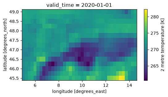
Optional: align the area of interest on chunk boundaries#
This a pro move and you can skip it.
When accessing the data in Zarr you always download whole chunks, even if you are only interested in part of them. In the case of ERA5 single level the spatial chunks are (60, 60) in size and even if you can read above that your DataArray in only 1.7GiB of data you are most probably downloading more data and then throwing a part of it away.
You can use the following (not very nice) code to grow your area of interest to the boundaries of the Zarr chunks, so you use all the data you download. Note that now you also have the size of the data that would be downloaded is it was not compressed (the data is in fact compressed so actual download is smaller).
[5]:
def align_indexer(step, indexer):
    if not isinstance(indexer, slice):
        return indexer
    assert indexer.step is None
    start = indexer.start // step * step if indexer.start else indexer.start
    stop = ((indexer.stop - 1) // step + 1) * step if indexer.stop else indexer.stop
    return slice(start, stop)


query_results = xr.core.indexing.map_index_queries(
    t2m_world, indexers=aoi_selection, method=None, tolerance=None
)
print(query_results.dim_indexers)

aoi_iselection = {
    dim: align_indexer(60, query_results.dim_indexers[dim])
    for dim in query_results.dim_indexers
}
print(aoi_iselection)

t2m_aoi = t2m_world.isel(aoi_iselection)
t2m_aoi
{'latitude': slice(164, 179, None), 'longitude': slice(20, 59, None)}
{'latitude': slice(120, 180, None), 'longitude': slice(0, 60, None)}
[5]:
<xarray.DataArray 't2m' (valid_time: 760440, latitude: 60, longitude: 60)> Size: 11GB
dask.array<getitem, shape=(760440, 60, 60), dtype=float32, chunksize=(1080, 60, 60), chunktype=numpy.ndarray>
Coordinates:
  * valid_time  (valid_time) datetime64[ns] 6MB 1940-01-01 ... 2026-09-30T23:...
  * latitude    (latitude) float64 480B 60.0 59.75 59.5 ... 45.75 45.5 45.25
  * longitude   (longitude) float64 480B 0.0 0.25 0.5 0.75 ... 14.25 14.5 14.75
Attributes: (12/32)
    GRIB_paramId:                             167
    GRIB_dataType:                            an
    GRIB_numberOfPoints:                      1038240
    GRIB_typeOfLevel:                         surface
    GRIB_stepUnits:                           1
    GRIB_stepType:                            instant
    ...                                       ...
    GRIB_totalNumber:                         0
    GRIB_units:                               K
    long_name:                                2 metre temperature
    units:                                    K
    standard_name:                            unknown
last_ingested_valid_time_index: 760439- valid_time: 760440
- latitude: 60
- longitude: 60
- dask.array<chunksize=(1080, 60, 60), meta=np.ndarray>
Array Chunk Bytes 10.20 GiB 14.83 MiB Shape (760440, 60, 60) (1080, 60, 60) Dask graph 705 chunks in 3 graph layers Data type float32 numpy.ndarray - valid_time(valid_time)datetime64[ns]1940-01-01 ... 2026-09-30T23:00:00
array(['1940-01-01T00:00:00.000000000', '1940-01-01T01:00:00.000000000', '1940-01-01T02:00:00.000000000', ..., '2026-09-30T21:00:00.000000000', '2026-09-30T22:00:00.000000000', '2026-09-30T23:00:00.000000000'], shape=(760440,), dtype='datetime64[ns]') - latitude(latitude)float6460.0 59.75 59.5 ... 45.5 45.25
- units :
- degrees_north
- standard_name :
- latitude
- long_name :
- latitude
- stored_direction :
- decreasing
array([60. , 59.75, 59.5 , 59.25, 59. , 58.75, 58.5 , 58.25, 58. , 57.75, 57.5 , 57.25, 57. , 56.75, 56.5 , 56.25, 56. , 55.75, 55.5 , 55.25, 55. , 54.75, 54.5 , 54.25, 54. , 53.75, 53.5 , 53.25, 53. , 52.75, 52.5 , 52.25, 52. , 51.75, 51.5 , 51.25, 51. , 50.75, 50.5 , 50.25, 50. , 49.75, 49.5 , 49.25, 49. , 48.75, 48.5 , 48.25, 48. , 47.75, 47.5 , 47.25, 47. , 46.75, 46.5 , 46.25, 46. , 45.75, 45.5 , 45.25]) - longitude(longitude)float640.0 0.25 0.5 ... 14.25 14.5 14.75
- units :
- degrees_east
- standard_name :
- longitude
- long_name :
- longitude
array([ 0.  ,  0.25,  0.5 ,  0.75,  1.  ,  1.25,  1.5 ,  1.75,  2.  ,  2.25,
        2.5 ,  2.75,  3.  ,  3.25,  3.5 ,  3.75,  4.  ,  4.25,  4.5 ,  4.75,
        5.  ,  5.25,  5.5 ,  5.75,  6.  ,  6.25,  6.5 ,  6.75,  7.  ,  7.25,
        7.5 ,  7.75,  8.  ,  8.25,  8.5 ,  8.75,  9.  ,  9.25,  9.5 ,  9.75,
       10.  , 10.25, 10.5 , 10.75, 11.  , 11.25, 11.5 , 11.75, 12.  , 12.25,
       12.5 , 12.75, 13.  , 13.25, 13.5 , 13.75, 14.  , 14.25, 14.5 , 14.75])
- GRIB_paramId :
- 167
- GRIB_dataType :
- an
- GRIB_numberOfPoints :
- 1038240
- GRIB_typeOfLevel :
- surface
- GRIB_stepUnits :
- 1
- GRIB_stepType :
- instant
- GRIB_gridType :
- regular_ll
- GRIB_uvRelativeToGrid :
- 0
- GRIB_NV :
- 0
- GRIB_Nx :
- 1440
- GRIB_Ny :
- 721
- GRIB_cfName :
- unknown
- GRIB_cfVarName :
- t2m
- GRIB_gridDefinitionDescription :
- Latitude/Longitude Grid
- GRIB_iDirectionIncrementInDegrees :
- 0.25
- GRIB_iScansNegatively :
- 0
- GRIB_jDirectionIncrementInDegrees :
- 0.25
- GRIB_jPointsAreConsecutive :
- 0
- GRIB_jScansPositively :
- 0
- GRIB_latitudeOfFirstGridPointInDegrees :
- 90.0
- GRIB_latitudeOfLastGridPointInDegrees :
- -90.0
- GRIB_longitudeOfFirstGridPointInDegrees :
- 0.0
- GRIB_longitudeOfLastGridPointInDegrees :
- 359.75
- GRIB_missingValue :
- 3.4028234663852886e+38
- GRIB_name :
- 2 metre temperature
- GRIB_shortName :
- 2t
- GRIB_totalNumber :
- 0
- GRIB_units :
- K
- long_name :
- 2 metre temperature
- units :
- K
- standard_name :
- unknown
- last_ingested_valid_time_index :
- 760439
So, the full time-series for a whole chunk is really 10GiB, not 1.7GiB.
Let’s have a look at the area of the whole chunk.
[6]:
t2m_aoi.sel(valid_time="2020-01-01T00:00:00").plot()
[6]:
<matplotlib.collections.QuadMesh at 0x1362dbd90>
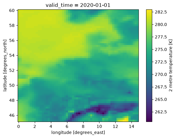
Great! A single 60x60 chunk gets a big part of central Europe.
Select the time interval of interest#
We take one of the typical 30 year periods to compute climatologies and finally we have a definition of the data we want to download.
[7]:
t2m_aoi_toi = t2m_aoi.sel(valid_time=slice("1981", "2010"))
t2m_aoi_toi
[7]:
<xarray.DataArray 't2m' (valid_time: 262968, latitude: 60, longitude: 60)> Size: 4GB
dask.array<getitem, shape=(262968, 60, 60), dtype=float32, chunksize=(1080, 60, 60), chunktype=numpy.ndarray>
Coordinates:
  * valid_time  (valid_time) datetime64[ns] 2MB 1981-01-01 ... 2010-12-31T23:...
  * latitude    (latitude) float64 480B 60.0 59.75 59.5 ... 45.75 45.5 45.25
  * longitude   (longitude) float64 480B 0.0 0.25 0.5 0.75 ... 14.25 14.5 14.75
Attributes: (12/32)
    GRIB_paramId:                             167
    GRIB_dataType:                            an
    GRIB_numberOfPoints:                      1038240
    GRIB_typeOfLevel:                         surface
    GRIB_stepUnits:                           1
    GRIB_stepType:                            instant
    ...                                       ...
    GRIB_totalNumber:                         0
    GRIB_units:                               K
    long_name:                                2 metre temperature
    units:                                    K
    standard_name:                            unknown
last_ingested_valid_time_index: 760439- valid_time: 262968
- latitude: 60
- longitude: 60
- dask.array<chunksize=(216, 60, 60), meta=np.ndarray>
Array Chunk Bytes 3.53 GiB 14.83 MiB Shape (262968, 60, 60) (1080, 60, 60) Dask graph 245 chunks in 4 graph layers Data type float32 numpy.ndarray - valid_time(valid_time)datetime64[ns]1981-01-01 ... 2010-12-31T23:00:00
array(['1981-01-01T00:00:00.000000000', '1981-01-01T01:00:00.000000000', '1981-01-01T02:00:00.000000000', ..., '2010-12-31T21:00:00.000000000', '2010-12-31T22:00:00.000000000', '2010-12-31T23:00:00.000000000'], shape=(262968,), dtype='datetime64[ns]') - latitude(latitude)float6460.0 59.75 59.5 ... 45.5 45.25
- units :
- degrees_north
- standard_name :
- latitude
- long_name :
- latitude
- stored_direction :
- decreasing
array([60. , 59.75, 59.5 , 59.25, 59. , 58.75, 58.5 , 58.25, 58. , 57.75, 57.5 , 57.25, 57. , 56.75, 56.5 , 56.25, 56. , 55.75, 55.5 , 55.25, 55. , 54.75, 54.5 , 54.25, 54. , 53.75, 53.5 , 53.25, 53. , 52.75, 52.5 , 52.25, 52. , 51.75, 51.5 , 51.25, 51. , 50.75, 50.5 , 50.25, 50. , 49.75, 49.5 , 49.25, 49. , 48.75, 48.5 , 48.25, 48. , 47.75, 47.5 , 47.25, 47. , 46.75, 46.5 , 46.25, 46. , 45.75, 45.5 , 45.25]) - longitude(longitude)float640.0 0.25 0.5 ... 14.25 14.5 14.75
- units :
- degrees_east
- standard_name :
- longitude
- long_name :
- longitude
array([ 0.  ,  0.25,  0.5 ,  0.75,  1.  ,  1.25,  1.5 ,  1.75,  2.  ,  2.25,
        2.5 ,  2.75,  3.  ,  3.25,  3.5 ,  3.75,  4.  ,  4.25,  4.5 ,  4.75,
        5.  ,  5.25,  5.5 ,  5.75,  6.  ,  6.25,  6.5 ,  6.75,  7.  ,  7.25,
        7.5 ,  7.75,  8.  ,  8.25,  8.5 ,  8.75,  9.  ,  9.25,  9.5 ,  9.75,
       10.  , 10.25, 10.5 , 10.75, 11.  , 11.25, 11.5 , 11.75, 12.  , 12.25,
       12.5 , 12.75, 13.  , 13.25, 13.5 , 13.75, 14.  , 14.25, 14.5 , 14.75])
- GRIB_paramId :
- 167
- GRIB_dataType :
- an
- GRIB_numberOfPoints :
- 1038240
- GRIB_typeOfLevel :
- surface
- GRIB_stepUnits :
- 1
- GRIB_stepType :
- instant
- GRIB_gridType :
- regular_ll
- GRIB_uvRelativeToGrid :
- 0
- GRIB_NV :
- 0
- GRIB_Nx :
- 1440
- GRIB_Ny :
- 721
- GRIB_cfName :
- unknown
- GRIB_cfVarName :
- t2m
- GRIB_gridDefinitionDescription :
- Latitude/Longitude Grid
- GRIB_iDirectionIncrementInDegrees :
- 0.25
- GRIB_iScansNegatively :
- 0
- GRIB_jDirectionIncrementInDegrees :
- 0.25
- GRIB_jPointsAreConsecutive :
- 0
- GRIB_jScansPositively :
- 0
- GRIB_latitudeOfFirstGridPointInDegrees :
- 90.0
- GRIB_latitudeOfLastGridPointInDegrees :
- -90.0
- GRIB_longitudeOfFirstGridPointInDegrees :
- 0.0
- GRIB_longitudeOfLastGridPointInDegrees :
- 359.75
- GRIB_missingValue :
- 3.4028234663852886e+38
- GRIB_name :
- 2 metre temperature
- GRIB_shortName :
- 2t
- GRIB_totalNumber :
- 0
- GRIB_units :
- K
- long_name :
- 2 metre temperature
- units :
- K
- standard_name :
- unknown
- last_ingested_valid_time_index :
- 760439
From the representation above we learn a few things:
the uncompressed data to be downloaded, e.g. 3.5GiB (compression depends on the dataset and the variable)
the number of chunks to be downloaded, e.g. 245
Download the data to memory#
Finally we are ready to download only the data that we are interested in, in memory.
The best practice is to call the .compute() method load the data into a numpy array in memory.
This operation is the slow one. It can take up to 10 minutes.
It depends on the download speed of your internet connection and on the load on the Earth Data Hub. The closer you are to the data the faster it is, and this is one of the reason the EDH is best suited to be used from within the DestinE platform.
[8]:
%%time

t2m_aoi_toi_data = t2m_aoi_toi.compute()
CPU times: user 20.7 s, sys: 6.2 s, total: 26.9 s
Wall time: 3min 55s
Perform any computation#
Prepare the raw data#
[9]:
t2m_aoi_toi_data_C = t2m_aoi_toi_data - 273.15
t2m_aoi_toi_data_C.attrs["units"] = "°C"
t2m_aoi_toi_data_C.attrs["long_name"] = "surface temperature"
t2m_aoi_toi_data_C
[9]:
<xarray.DataArray 't2m' (valid_time: 262968, latitude: 60, longitude: 60)> Size: 4GB
array([[[ 4.100006 ,  4.100006 ,  3.850006 , ...,  0.3500061,
          0.3500061,  0.3500061],
        [ 3.850006 ,  3.850006 ,  3.850006 , ...,  0.3500061,
          0.3500061,  0.3500061],
        [ 3.850006 ,  4.100006 ,  4.350006 , ...,  0.6000061,
          0.6000061,  0.6000061],
        ...,
        [ 3.350006 ,  3.100006 ,  2.600006 , ..., -4.649994 ,
         -5.649994 , -6.399994 ],
        [ 3.350006 ,  2.850006 ,  2.600006 , ...,  0.6000061,
         -0.6499939, -1.6499939],
        [ 3.100006 ,  2.850006 ,  2.600006 , ...,  6.100006 ,
          4.850006 ,  1.6000061]],

       [[ 4.100006 ,  4.100006 ,  4.100006 , ...,  0.1000061,
          0.1000061,  0.3500061],
        [ 4.100006 ,  4.100006 ,  4.100006 , ...,  0.1000061,
          0.1000061,  0.3500061],
        [ 3.850006 ,  3.850006 ,  3.850006 , ...,  0.6000061,
          0.6000061,  0.8500061],
...
        [ 5.600006 ,  5.850006 ,  6.100006 , ..., -2.149994 ,
         -2.649994 , -4.149994 ],
        [ 5.600006 ,  5.600006 ,  5.850006 , ..., -1.8999939,
         -4.149994 , -5.649994 ],
        [ 6.100006 ,  6.350006 ,  6.350006 , ...,  2.100006 ,
         -0.3999939, -3.649994 ]],

       [[ 5.100006 ,  5.100006 ,  5.100006 , ..., -1.3999939,
         -1.1499939, -0.8999939],
        [ 5.100006 ,  5.100006 ,  5.100006 , ..., -0.3999939,
         -0.3999939, -0.1499939],
        [ 5.100006 ,  5.100006 ,  5.100006 , ...,  0.1000061,
          0.3500061,  0.6000061],
        ...,
        [ 5.100006 ,  5.350006 ,  5.600006 , ..., -2.399994 ,
         -2.399994 , -3.649994 ],
        [ 5.100006 ,  5.350006 ,  5.600006 , ..., -1.8999939,
         -3.899994 , -5.399994 ],
        [ 5.350006 ,  5.600006 ,  5.850006 , ...,  1.8500061,
         -0.6499939, -3.649994 ]]], shape=(262968, 60, 60), dtype=float32)
Coordinates:
  * valid_time  (valid_time) datetime64[ns] 2MB 1981-01-01 ... 2010-12-31T23:...
  * latitude    (latitude) float64 480B 60.0 59.75 59.5 ... 45.75 45.5 45.25
  * longitude   (longitude) float64 480B 0.0 0.25 0.5 0.75 ... 14.25 14.5 14.75
Attributes: (12/32)
    GRIB_paramId:                             167
    GRIB_dataType:                            an
    GRIB_numberOfPoints:                      1038240
    GRIB_typeOfLevel:                         surface
    GRIB_stepUnits:                           1
    GRIB_stepType:                            instant
    ...                                       ...
    GRIB_totalNumber:                         0
    GRIB_units:                               K
    long_name:                                surface temperature
    units:                                    °C
    standard_name:                            unknown
last_ingested_valid_time_index: 760439- valid_time: 262968
- latitude: 60
- longitude: 60
- 4.1 4.1 3.85 3.85 3.6 3.85 3.85 ... 7.85 7.6 2.85 2.1 1.85 -0.65 -3.65
array([[[ 4.100006 , 4.100006 , 3.850006 , ..., 0.3500061, 0.3500061, 0.3500061], [ 3.850006 , 3.850006 , 3.850006 , ..., 0.3500061, 0.3500061, 0.3500061], [ 3.850006 , 4.100006 , 4.350006 , ..., 0.6000061, 0.6000061, 0.6000061], ..., [ 3.350006 , 3.100006 , 2.600006 , ..., -4.649994 , -5.649994 , -6.399994 ], [ 3.350006 , 2.850006 , 2.600006 , ..., 0.6000061, -0.6499939, -1.6499939], [ 3.100006 , 2.850006 , 2.600006 , ..., 6.100006 , 4.850006 , 1.6000061]], [[ 4.100006 , 4.100006 , 4.100006 , ..., 0.1000061, 0.1000061, 0.3500061], [ 4.100006 , 4.100006 , 4.100006 , ..., 0.1000061, 0.1000061, 0.3500061], [ 3.850006 , 3.850006 , 3.850006 , ..., 0.6000061, 0.6000061, 0.8500061], ... [ 5.600006 , 5.850006 , 6.100006 , ..., -2.149994 , -2.649994 , -4.149994 ], [ 5.600006 , 5.600006 , 5.850006 , ..., -1.8999939, -4.149994 , -5.649994 ], [ 6.100006 , 6.350006 , 6.350006 , ..., 2.100006 , -0.3999939, -3.649994 ]], [[ 5.100006 , 5.100006 , 5.100006 , ..., -1.3999939, -1.1499939, -0.8999939], [ 5.100006 , 5.100006 , 5.100006 , ..., -0.3999939, -0.3999939, -0.1499939], [ 5.100006 , 5.100006 , 5.100006 , ..., 0.1000061, 0.3500061, 0.6000061], ..., [ 5.100006 , 5.350006 , 5.600006 , ..., -2.399994 , -2.399994 , -3.649994 ], [ 5.100006 , 5.350006 , 5.600006 , ..., -1.8999939, -3.899994 , -5.399994 ], [ 5.350006 , 5.600006 , 5.850006 , ..., 1.8500061, -0.6499939, -3.649994 ]]], shape=(262968, 60, 60), dtype=float32) - valid_time(valid_time)datetime64[ns]1981-01-01 ... 2010-12-31T23:00:00
array(['1981-01-01T00:00:00.000000000', '1981-01-01T01:00:00.000000000', '1981-01-01T02:00:00.000000000', ..., '2010-12-31T21:00:00.000000000', '2010-12-31T22:00:00.000000000', '2010-12-31T23:00:00.000000000'], shape=(262968,), dtype='datetime64[ns]') - latitude(latitude)float6460.0 59.75 59.5 ... 45.5 45.25
- units :
- degrees_north
- standard_name :
- latitude
- long_name :
- latitude
- stored_direction :
- decreasing
array([60. , 59.75, 59.5 , 59.25, 59. , 58.75, 58.5 , 58.25, 58. , 57.75, 57.5 , 57.25, 57. , 56.75, 56.5 , 56.25, 56. , 55.75, 55.5 , 55.25, 55. , 54.75, 54.5 , 54.25, 54. , 53.75, 53.5 , 53.25, 53. , 52.75, 52.5 , 52.25, 52. , 51.75, 51.5 , 51.25, 51. , 50.75, 50.5 , 50.25, 50. , 49.75, 49.5 , 49.25, 49. , 48.75, 48.5 , 48.25, 48. , 47.75, 47.5 , 47.25, 47. , 46.75, 46.5 , 46.25, 46. , 45.75, 45.5 , 45.25]) - longitude(longitude)float640.0 0.25 0.5 ... 14.25 14.5 14.75
- units :
- degrees_east
- standard_name :
- longitude
- long_name :
- longitude
array([ 0.  ,  0.25,  0.5 ,  0.75,  1.  ,  1.25,  1.5 ,  1.75,  2.  ,  2.25,
        2.5 ,  2.75,  3.  ,  3.25,  3.5 ,  3.75,  4.  ,  4.25,  4.5 ,  4.75,
        5.  ,  5.25,  5.5 ,  5.75,  6.  ,  6.25,  6.5 ,  6.75,  7.  ,  7.25,
        7.5 ,  7.75,  8.  ,  8.25,  8.5 ,  8.75,  9.  ,  9.25,  9.5 ,  9.75,
       10.  , 10.25, 10.5 , 10.75, 11.  , 11.25, 11.5 , 11.75, 12.  , 12.25,
       12.5 , 12.75, 13.  , 13.25, 13.5 , 13.75, 14.  , 14.25, 14.5 , 14.75])
- GRIB_paramId :
- 167
- GRIB_dataType :
- an
- GRIB_numberOfPoints :
- 1038240
- GRIB_typeOfLevel :
- surface
- GRIB_stepUnits :
- 1
- GRIB_stepType :
- instant
- GRIB_gridType :
- regular_ll
- GRIB_uvRelativeToGrid :
- 0
- GRIB_NV :
- 0
- GRIB_Nx :
- 1440
- GRIB_Ny :
- 721
- GRIB_cfName :
- unknown
- GRIB_cfVarName :
- t2m
- GRIB_gridDefinitionDescription :
- Latitude/Longitude Grid
- GRIB_iDirectionIncrementInDegrees :
- 0.25
- GRIB_iScansNegatively :
- 0
- GRIB_jDirectionIncrementInDegrees :
- 0.25
- GRIB_jPointsAreConsecutive :
- 0
- GRIB_jScansPositively :
- 0
- GRIB_latitudeOfFirstGridPointInDegrees :
- 90.0
- GRIB_latitudeOfLastGridPointInDegrees :
- -90.0
- GRIB_longitudeOfFirstGridPointInDegrees :
- 0.0
- GRIB_longitudeOfLastGridPointInDegrees :
- 359.75
- GRIB_missingValue :
- 3.4028234663852886e+38
- GRIB_name :
- 2 metre temperature
- GRIB_shortName :
- 2t
- GRIB_totalNumber :
- 0
- GRIB_units :
- K
- long_name :
- surface temperature
- units :
- °C
- standard_name :
- unknown
- last_ingested_valid_time_index :
- 760439
Monthly climatology#
[10]:
%%time

t2m_aoi_toi_month_mean = t2m_aoi_toi_data_C.groupby("valid_time.month").mean()
t2m_aoi_toi_month_mean
CPU times: user 1.42 s, sys: 1.56 s, total: 2.97 s
Wall time: 3.3 s
[10]:
<xarray.DataArray 't2m' (month: 12, latitude: 60, longitude: 60)> Size: 173kB
array([[[ 5.9818087 ,  5.9669843 ,  5.9524713 , ..., -4.6589036 ,
         -4.6404414 , -4.5902905 ],
        [ 5.966629  ,  5.9526863 ,  5.939012  , ..., -4.094842  ,
         -4.065144  , -3.9923122 ],
        [ 6.005804  ,  5.9744687 ,  5.9492054 , ..., -3.5102892 ,
         -3.5077865 , -3.4893947 ],
        ...,
        [ 5.372132  ,  5.2229385 ,  4.908522  , ..., -0.54323304,
         -0.6738021 , -0.7514413 ],
        [ 5.3958364 ,  5.315269  ,  4.998812  , ...,  0.5302754 ,
         -0.5924382 , -0.66884124],
        [ 5.5873632 ,  5.500552  ,  5.268542  , ...,  3.7213507 ,
          2.4584892 ,  0.1901969 ]],

       [[ 5.435061  ,  5.423069  ,  5.411557  , ..., -4.5158525 ,
         -4.515467  , -4.454127  ],
        [ 5.4172597 ,  5.404431  ,  5.390594  , ..., -3.9671335 ,
         -3.9808495 , -3.9163103 ],
        [ 5.449186  ,  5.420084  ,  5.3954844 , ..., -3.480913  ,
         -3.50844   , -3.4638371 ],
...
        [ 8.523972  ,  8.35806   ,  8.028974  , ...,  4.6578    ,
          4.5535216 ,  4.527012  ],
        [ 8.590157  ,  8.537646  ,  8.20685   , ...,  5.6508393 ,
          4.6596746 ,  4.6317544 ],
        [ 8.833831  ,  8.77931   ,  8.573055  , ...,  8.549518  ,
          7.447578  ,  5.4716263 ]],

       [[ 6.4842925 ,  6.4615417 ,  6.43884   , ..., -3.8836484 ,
         -3.8491683 , -3.776545  ],
        [ 6.469015  ,  6.4461217 ,  6.426031  , ..., -3.2930243 ,
         -3.2093337 , -3.113703  ],
        [ 6.519353  ,  6.482286  ,  6.4501595 , ..., -2.6695938 ,
         -2.6275818 , -2.6314178 ],
        ...,
        [ 5.94075   ,  5.8095894 ,  5.5204873 , ...,  0.6526263 ,
          0.48733467,  0.37250245],
        [ 5.992099  ,  5.9452276 ,  5.653638  , ...,  1.6936718 ,
          0.6220236 ,  0.508619  ],
        [ 6.1915736 ,  6.135068  ,  5.917882  , ...,  4.9268003 ,
          3.711836  ,  1.4372185 ]]], shape=(12, 60, 60), dtype=float32)
Coordinates:
  * month      (month) int64 96B 1 2 3 4 5 6 7 8 9 10 11 12
  * latitude   (latitude) float64 480B 60.0 59.75 59.5 ... 45.75 45.5 45.25
  * longitude  (longitude) float64 480B 0.0 0.25 0.5 0.75 ... 14.25 14.5 14.75
Attributes: (12/32)
    GRIB_paramId:                             167
    GRIB_dataType:                            an
    GRIB_numberOfPoints:                      1038240
    GRIB_typeOfLevel:                         surface
    GRIB_stepUnits:                           1
    GRIB_stepType:                            instant
    ...                                       ...
    GRIB_totalNumber:                         0
    GRIB_units:                               K
    long_name:                                surface temperature
    units:                                    °C
    standard_name:                            unknown
last_ingested_valid_time_index: 760439- month: 12
- latitude: 60
- longitude: 60
- 5.982 5.967 5.952 5.89 5.82 5.781 ... 6.174 5.641 4.927 3.712 1.437
array([[[ 5.9818087 , 5.9669843 , 5.9524713 , ..., -4.6589036 , -4.6404414 , -4.5902905 ], [ 5.966629 , 5.9526863 , 5.939012 , ..., -4.094842 , -4.065144 , -3.9923122 ], [ 6.005804 , 5.9744687 , 5.9492054 , ..., -3.5102892 , -3.5077865 , -3.4893947 ], ..., [ 5.372132 , 5.2229385 , 4.908522 , ..., -0.54323304, -0.6738021 , -0.7514413 ], [ 5.3958364 , 5.315269 , 4.998812 , ..., 0.5302754 , -0.5924382 , -0.66884124], [ 5.5873632 , 5.500552 , 5.268542 , ..., 3.7213507 , 2.4584892 , 0.1901969 ]], [[ 5.435061 , 5.423069 , 5.411557 , ..., -4.5158525 , -4.515467 , -4.454127 ], [ 5.4172597 , 5.404431 , 5.390594 , ..., -3.9671335 , -3.9808495 , -3.9163103 ], [ 5.449186 , 5.420084 , 5.3954844 , ..., -3.480913 , -3.50844 , -3.4638371 ], ... [ 8.523972 , 8.35806 , 8.028974 , ..., 4.6578 , 4.5535216 , 4.527012 ], [ 8.590157 , 8.537646 , 8.20685 , ..., 5.6508393 , 4.6596746 , 4.6317544 ], [ 8.833831 , 8.77931 , 8.573055 , ..., 8.549518 , 7.447578 , 5.4716263 ]], [[ 6.4842925 , 6.4615417 , 6.43884 , ..., -3.8836484 , -3.8491683 , -3.776545 ], [ 6.469015 , 6.4461217 , 6.426031 , ..., -3.2930243 , -3.2093337 , -3.113703 ], [ 6.519353 , 6.482286 , 6.4501595 , ..., -2.6695938 , -2.6275818 , -2.6314178 ], ..., [ 5.94075 , 5.8095894 , 5.5204873 , ..., 0.6526263 , 0.48733467, 0.37250245], [ 5.992099 , 5.9452276 , 5.653638 , ..., 1.6936718 , 0.6220236 , 0.508619 ], [ 6.1915736 , 6.135068 , 5.917882 , ..., 4.9268003 , 3.711836 , 1.4372185 ]]], shape=(12, 60, 60), dtype=float32) - month(month)int641 2 3 4 5 6 7 8 9 10 11 12
array([ 1, 2, 3, 4, 5, 6, 7, 8, 9, 10, 11, 12])
- latitude(latitude)float6460.0 59.75 59.5 ... 45.5 45.25
- units :
- degrees_north
- standard_name :
- latitude
- long_name :
- latitude
- stored_direction :
- decreasing
array([60. , 59.75, 59.5 , 59.25, 59. , 58.75, 58.5 , 58.25, 58. , 57.75, 57.5 , 57.25, 57. , 56.75, 56.5 , 56.25, 56. , 55.75, 55.5 , 55.25, 55. , 54.75, 54.5 , 54.25, 54. , 53.75, 53.5 , 53.25, 53. , 52.75, 52.5 , 52.25, 52. , 51.75, 51.5 , 51.25, 51. , 50.75, 50.5 , 50.25, 50. , 49.75, 49.5 , 49.25, 49. , 48.75, 48.5 , 48.25, 48. , 47.75, 47.5 , 47.25, 47. , 46.75, 46.5 , 46.25, 46. , 45.75, 45.5 , 45.25]) - longitude(longitude)float640.0 0.25 0.5 ... 14.25 14.5 14.75
- units :
- degrees_east
- standard_name :
- longitude
- long_name :
- longitude
array([ 0.  ,  0.25,  0.5 ,  0.75,  1.  ,  1.25,  1.5 ,  1.75,  2.  ,  2.25,
        2.5 ,  2.75,  3.  ,  3.25,  3.5 ,  3.75,  4.  ,  4.25,  4.5 ,  4.75,
        5.  ,  5.25,  5.5 ,  5.75,  6.  ,  6.25,  6.5 ,  6.75,  7.  ,  7.25,
        7.5 ,  7.75,  8.  ,  8.25,  8.5 ,  8.75,  9.  ,  9.25,  9.5 ,  9.75,
       10.  , 10.25, 10.5 , 10.75, 11.  , 11.25, 11.5 , 11.75, 12.  , 12.25,
       12.5 , 12.75, 13.  , 13.25, 13.5 , 13.75, 14.  , 14.25, 14.5 , 14.75])
- GRIB_paramId :
- 167
- GRIB_dataType :
- an
- GRIB_numberOfPoints :
- 1038240
- GRIB_typeOfLevel :
- surface
- GRIB_stepUnits :
- 1
- GRIB_stepType :
- instant
- GRIB_gridType :
- regular_ll
- GRIB_uvRelativeToGrid :
- 0
- GRIB_NV :
- 0
- GRIB_Nx :
- 1440
- GRIB_Ny :
- 721
- GRIB_cfName :
- unknown
- GRIB_cfVarName :
- t2m
- GRIB_gridDefinitionDescription :
- Latitude/Longitude Grid
- GRIB_iDirectionIncrementInDegrees :
- 0.25
- GRIB_iScansNegatively :
- 0
- GRIB_jDirectionIncrementInDegrees :
- 0.25
- GRIB_jPointsAreConsecutive :
- 0
- GRIB_jScansPositively :
- 0
- GRIB_latitudeOfFirstGridPointInDegrees :
- 90.0
- GRIB_latitudeOfLastGridPointInDegrees :
- -90.0
- GRIB_longitudeOfFirstGridPointInDegrees :
- 0.0
- GRIB_longitudeOfLastGridPointInDegrees :
- 359.75
- GRIB_missingValue :
- 3.4028234663852886e+38
- GRIB_name :
- 2 metre temperature
- GRIB_shortName :
- 2t
- GRIB_totalNumber :
- 0
- GRIB_units :
- K
- long_name :
- surface temperature
- units :
- °C
- standard_name :
- unknown
- last_ingested_valid_time_index :
- 760439
[11]:
t2m_aoi_toi_month_mean.plot(vmin=-30, col="month", col_wrap=3)
[11]:
<xarray.plot.facetgrid.FacetGrid at 0x136444d70>
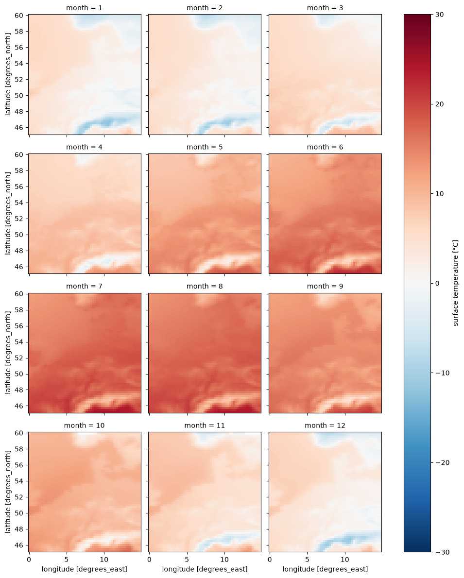
Daily climatological mean and quintile extremes#
[12]:
%%time

t2m_aoi_toi_doy_mean = t2m_aoi_toi_data_C.groupby("valid_time.dayofyear").mean()
t2m_aoi_toi_doy_mean = t2m_aoi_toi_doy_mean.sel(dayofyear=slice(0, 365))
t2m_aoi_toi_doy_mean
CPU times: user 1.28 s, sys: 519 ms, total: 1.8 s
Wall time: 1.82 s
[12]:
<xarray.DataArray 't2m' (dayofyear: 365, latitude: 60, longitude: 60)> Size: 5MB
array([[[ 5.904207  ,  5.870874  ,  5.839971  , ..., -5.089555  ,
         -5.082957  , -5.0829525 ],
        [ 5.8865    ,  5.862889  ,  5.8344164 , ..., -4.3419957 ,
         -4.3058844 , -4.2820997 ],
        [ 5.927126  ,  5.8861523 ,  5.8514304 , ..., -3.6145732 ,
         -3.6137052 , -3.6147463 ],
        ...,
        [ 5.1840544 ,  4.9882197 ,  4.6434255 , ..., -0.07325779,
         -0.28298035, -0.45034602],
        [ 5.2830133 ,  5.1284995 ,  4.779885  , ...,  1.1416657 ,
         -0.02152167, -0.18749389],
        [ 5.514266  ,  5.3503757 ,  5.0739846 , ...,  4.3979406 ,
          3.1308913 ,  0.9215325 ]],

       [[ 5.8250422 ,  5.791014  ,  5.7660136 , ..., -6.0864205 ,
         -6.0947537 , -6.0570803 ],
        [ 5.828862  ,  5.8003893 ,  5.784417  , ..., -5.4367695 ,
         -5.3806934 , -5.331736  ],
        [ 5.8896275 ,  5.8524737 ,  5.819487  , ..., -4.756582  ,
         -4.7326236 , -4.76995   ],
...
        [ 5.352464  ,  5.2437835 ,  5.005241  , ..., -0.36804944,
         -0.4121467 , -0.467355  ],
        [ 5.4253807 ,  5.404895  ,  5.1607966 , ...,  0.6833377 ,
         -0.46388277, -0.5246467 ],
        [ 5.683368  ,  5.6465626 ,  5.4590616 , ...,  3.9409862 ,
          2.644079  ,  0.34861723]],

       [[ 6.063586  ,  6.038239  ,  6.00942   , ..., -6.568361  ,
         -6.481903  , -6.380514  ],
        [ 6.0705314 ,  6.0451837 ,  6.032684  , ..., -5.656569  ,
         -5.4834795 , -5.3484106 ],
        [ 6.1399765 ,  6.1094213 ,  6.0799065 , ..., -4.6952934 ,
         -4.568905  , -4.5409536 ],
        ...,
        [ 5.254198  ,  5.155934  ,  4.9451675 , ..., -0.24929945,
         -0.3888828 , -0.5569388 ],
        [ 5.2965593 ,  5.3062816 ,  5.0916963 , ...,  0.91354203,
         -0.30034113, -0.46023697],
        [ 5.509407  ,  5.5073237 ,  5.38649   , ...,  4.1562657 ,
          2.8041487 ,  0.5128533 ]]], shape=(365, 60, 60), dtype=float32)
Coordinates:
  * dayofyear  (dayofyear) int64 3kB 1 2 3 4 5 6 7 ... 360 361 362 363 364 365
  * latitude   (latitude) float64 480B 60.0 59.75 59.5 ... 45.75 45.5 45.25
  * longitude  (longitude) float64 480B 0.0 0.25 0.5 0.75 ... 14.25 14.5 14.75
Attributes: (12/32)
    GRIB_paramId:                             167
    GRIB_dataType:                            an
    GRIB_numberOfPoints:                      1038240
    GRIB_typeOfLevel:                         surface
    GRIB_stepUnits:                           1
    GRIB_stepType:                            instant
    ...                                       ...
    GRIB_totalNumber:                         0
    GRIB_units:                               K
    long_name:                                surface temperature
    units:                                    °C
    standard_name:                            unknown
last_ingested_valid_time_index: 760439- dayofyear: 365
- latitude: 60
- longitude: 60
- 5.904 5.871 5.84 5.777 5.699 5.658 ... 5.395 4.859 4.156 2.804 0.5129
array([[[ 5.904207 , 5.870874 , 5.839971 , ..., -5.089555 , -5.082957 , -5.0829525 ], [ 5.8865 , 5.862889 , 5.8344164 , ..., -4.3419957 , -4.3058844 , -4.2820997 ], [ 5.927126 , 5.8861523 , 5.8514304 , ..., -3.6145732 , -3.6137052 , -3.6147463 ], ..., [ 5.1840544 , 4.9882197 , 4.6434255 , ..., -0.07325779, -0.28298035, -0.45034602], [ 5.2830133 , 5.1284995 , 4.779885 , ..., 1.1416657 , -0.02152167, -0.18749389], [ 5.514266 , 5.3503757 , 5.0739846 , ..., 4.3979406 , 3.1308913 , 0.9215325 ]], [[ 5.8250422 , 5.791014 , 5.7660136 , ..., -6.0864205 , -6.0947537 , -6.0570803 ], [ 5.828862 , 5.8003893 , 5.784417 , ..., -5.4367695 , -5.3806934 , -5.331736 ], [ 5.8896275 , 5.8524737 , 5.819487 , ..., -4.756582 , -4.7326236 , -4.76995 ], ... [ 5.352464 , 5.2437835 , 5.005241 , ..., -0.36804944, -0.4121467 , -0.467355 ], [ 5.4253807 , 5.404895 , 5.1607966 , ..., 0.6833377 , -0.46388277, -0.5246467 ], [ 5.683368 , 5.6465626 , 5.4590616 , ..., 3.9409862 , 2.644079 , 0.34861723]], [[ 6.063586 , 6.038239 , 6.00942 , ..., -6.568361 , -6.481903 , -6.380514 ], [ 6.0705314 , 6.0451837 , 6.032684 , ..., -5.656569 , -5.4834795 , -5.3484106 ], [ 6.1399765 , 6.1094213 , 6.0799065 , ..., -4.6952934 , -4.568905 , -4.5409536 ], ..., [ 5.254198 , 5.155934 , 4.9451675 , ..., -0.24929945, -0.3888828 , -0.5569388 ], [ 5.2965593 , 5.3062816 , 5.0916963 , ..., 0.91354203, -0.30034113, -0.46023697], [ 5.509407 , 5.5073237 , 5.38649 , ..., 4.1562657 , 2.8041487 , 0.5128533 ]]], shape=(365, 60, 60), dtype=float32) - dayofyear(dayofyear)int641 2 3 4 5 6 ... 361 362 363 364 365
array([ 1, 2, 3, ..., 363, 364, 365], shape=(365,))
- latitude(latitude)float6460.0 59.75 59.5 ... 45.5 45.25
- units :
- degrees_north
- standard_name :
- latitude
- long_name :
- latitude
- stored_direction :
- decreasing
array([60. , 59.75, 59.5 , 59.25, 59. , 58.75, 58.5 , 58.25, 58. , 57.75, 57.5 , 57.25, 57. , 56.75, 56.5 , 56.25, 56. , 55.75, 55.5 , 55.25, 55. , 54.75, 54.5 , 54.25, 54. , 53.75, 53.5 , 53.25, 53. , 52.75, 52.5 , 52.25, 52. , 51.75, 51.5 , 51.25, 51. , 50.75, 50.5 , 50.25, 50. , 49.75, 49.5 , 49.25, 49. , 48.75, 48.5 , 48.25, 48. , 47.75, 47.5 , 47.25, 47. , 46.75, 46.5 , 46.25, 46. , 45.75, 45.5 , 45.25]) - longitude(longitude)float640.0 0.25 0.5 ... 14.25 14.5 14.75
- units :
- degrees_east
- standard_name :
- longitude
- long_name :
- longitude
array([ 0.  ,  0.25,  0.5 ,  0.75,  1.  ,  1.25,  1.5 ,  1.75,  2.  ,  2.25,
        2.5 ,  2.75,  3.  ,  3.25,  3.5 ,  3.75,  4.  ,  4.25,  4.5 ,  4.75,
        5.  ,  5.25,  5.5 ,  5.75,  6.  ,  6.25,  6.5 ,  6.75,  7.  ,  7.25,
        7.5 ,  7.75,  8.  ,  8.25,  8.5 ,  8.75,  9.  ,  9.25,  9.5 ,  9.75,
       10.  , 10.25, 10.5 , 10.75, 11.  , 11.25, 11.5 , 11.75, 12.  , 12.25,
       12.5 , 12.75, 13.  , 13.25, 13.5 , 13.75, 14.  , 14.25, 14.5 , 14.75])
- GRIB_paramId :
- 167
- GRIB_dataType :
- an
- GRIB_numberOfPoints :
- 1038240
- GRIB_typeOfLevel :
- surface
- GRIB_stepUnits :
- 1
- GRIB_stepType :
- instant
- GRIB_gridType :
- regular_ll
- GRIB_uvRelativeToGrid :
- 0
- GRIB_NV :
- 0
- GRIB_Nx :
- 1440
- GRIB_Ny :
- 721
- GRIB_cfName :
- unknown
- GRIB_cfVarName :
- t2m
- GRIB_gridDefinitionDescription :
- Latitude/Longitude Grid
- GRIB_iDirectionIncrementInDegrees :
- 0.25
- GRIB_iScansNegatively :
- 0
- GRIB_jDirectionIncrementInDegrees :
- 0.25
- GRIB_jPointsAreConsecutive :
- 0
- GRIB_jScansPositively :
- 0
- GRIB_latitudeOfFirstGridPointInDegrees :
- 90.0
- GRIB_latitudeOfLastGridPointInDegrees :
- -90.0
- GRIB_longitudeOfFirstGridPointInDegrees :
- 0.0
- GRIB_longitudeOfLastGridPointInDegrees :
- 359.75
- GRIB_missingValue :
- 3.4028234663852886e+38
- GRIB_name :
- 2 metre temperature
- GRIB_shortName :
- 2t
- GRIB_totalNumber :
- 0
- GRIB_units :
- K
- long_name :
- surface temperature
- units :
- °C
- standard_name :
- unknown
- last_ingested_valid_time_index :
- 760439
[13]:
point = {
    "latitude": 46.5,
    "longitude": 11.8,
    "method": "nearest",
}

t2m_point_doy_mean = t2m_aoi_toi_doy_mean.sel(**point)

t2m_point_doy_mean.plot()
[13]:
[<matplotlib.lines.Line2D at 0x133f6c6e0>]
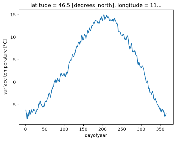
[14]:
%%time

t2m_aoi_toi_doy_quantile = t2m_aoi_toi_data_C.groupby("valid_time.dayofyear").quantile(
    [0.9, 0.5, 0.1]
)
t2m_aoi_toi_doy_quantile = t2m_aoi_toi_doy_quantile.sel(dayofyear=slice(0, 365))
t2m_aoi_toi_doy_quantile
CPU times: user 35.6 s, sys: 406 ms, total: 36 s
Wall time: 36.1 s
[14]:
<xarray.DataArray 't2m' (dayofyear: 365, latitude: 60, longitude: 60,
                         quantile: 3)> Size: 32MB
array([[[[  8.1000061,   6.1000061,   3.3500061],
         [  8.1000061,   5.8500061,   3.3500061],
         [  8.1000061,   5.8500061,   3.3500061],
         ...,
         [  2.3500061,  -4.1499939, -12.9249939],
         [  2.1000061,  -4.1499939, -12.4249939],
         [  2.1000061,  -4.1499939, -12.4249939]],

        [[  8.1000061,   5.8500061,   3.6000061],
         [  8.1000061,   5.8500061,   3.3500061],
         [  8.1000061,   5.8500061,   3.3500061],
         ...,
         [  2.8500061,  -3.3999939, -11.1499939],
         [  2.6000061,  -3.3999939, -10.6499939],
         [  2.8500061,  -3.3999939, -10.3999939]],

        [[  8.1000061,   5.9750061,   3.6000061],
         [  8.1000061,   5.8500061,   3.6000061],
         [  8.1000061,   5.8500061,   3.3500061],
         ...,
...
         [  6.3500061,  -0.1499939,  -6.1499939],
         [  6.3500061,  -0.3999939,  -6.8999939],
         [  6.6000061,  -0.3999939,  -7.1499939]],

        [[ 11.3500061,   6.6000061,  -2.1499939],
         [ 11.1000061,   6.6000061,  -1.8999939],
         [ 10.6000061,   6.3500061,  -1.6749939],
         ...,
         [  7.1000061,   1.1000061,  -4.8999939],
         [  6.8500061,   0.1000061,  -7.6499939],
         [  6.6000061,  -0.1499939,  -7.6749939]],

        [[ 11.6000061,   6.6000061,  -1.6499939],
         [ 11.1250061,   6.8500061,  -1.4249939],
         [ 10.8500061,   6.8500061,  -1.3999939],
         ...,
         [  9.3500061,   4.2250061,   0.0750061],
         [  8.8750061,   3.1000061,  -3.1499939],
         [  7.8500061,   0.8500061,  -6.8999939]]]],
      shape=(365, 60, 60, 3))
Coordinates:
  * dayofyear  (dayofyear) int64 3kB 1 2 3 4 5 6 7 ... 360 361 362 363 364 365
  * latitude   (latitude) float64 480B 60.0 59.75 59.5 ... 45.75 45.5 45.25
  * longitude  (longitude) float64 480B 0.0 0.25 0.5 0.75 ... 14.25 14.5 14.75
  * quantile   (quantile) float64 24B 0.9 0.5 0.1
Attributes: (12/32)
    GRIB_paramId:                             167
    GRIB_dataType:                            an
    GRIB_numberOfPoints:                      1038240
    GRIB_typeOfLevel:                         surface
    GRIB_stepUnits:                           1
    GRIB_stepType:                            instant
    ...                                       ...
    GRIB_totalNumber:                         0
    GRIB_units:                               K
    long_name:                                surface temperature
    units:                                    °C
    standard_name:                            unknown
last_ingested_valid_time_index: 760439- dayofyear: 365
- latitude: 60
- longitude: 60
- quantile: 3
- 8.1 6.1 3.35 8.1 5.85 3.35 8.1 ... 8.875 3.1 -3.15 7.85 0.85 -6.9
array([[[[ 8.1000061, 6.1000061, 3.3500061], [ 8.1000061, 5.8500061, 3.3500061], [ 8.1000061, 5.8500061, 3.3500061], ..., [ 2.3500061, -4.1499939, -12.9249939], [ 2.1000061, -4.1499939, -12.4249939], [ 2.1000061, -4.1499939, -12.4249939]], [[ 8.1000061, 5.8500061, 3.6000061], [ 8.1000061, 5.8500061, 3.3500061], [ 8.1000061, 5.8500061, 3.3500061], ..., [ 2.8500061, -3.3999939, -11.1499939], [ 2.6000061, -3.3999939, -10.6499939], [ 2.8500061, -3.3999939, -10.3999939]], [[ 8.1000061, 5.9750061, 3.6000061], [ 8.1000061, 5.8500061, 3.6000061], [ 8.1000061, 5.8500061, 3.3500061], ..., ... [ 6.3500061, -0.1499939, -6.1499939], [ 6.3500061, -0.3999939, -6.8999939], [ 6.6000061, -0.3999939, -7.1499939]], [[ 11.3500061, 6.6000061, -2.1499939], [ 11.1000061, 6.6000061, -1.8999939], [ 10.6000061, 6.3500061, -1.6749939], ..., [ 7.1000061, 1.1000061, -4.8999939], [ 6.8500061, 0.1000061, -7.6499939], [ 6.6000061, -0.1499939, -7.6749939]], [[ 11.6000061, 6.6000061, -1.6499939], [ 11.1250061, 6.8500061, -1.4249939], [ 10.8500061, 6.8500061, -1.3999939], ..., [ 9.3500061, 4.2250061, 0.0750061], [ 8.8750061, 3.1000061, -3.1499939], [ 7.8500061, 0.8500061, -6.8999939]]]], shape=(365, 60, 60, 3)) - dayofyear(dayofyear)int641 2 3 4 5 6 ... 361 362 363 364 365
array([ 1, 2, 3, ..., 363, 364, 365], shape=(365,))
- latitude(latitude)float6460.0 59.75 59.5 ... 45.5 45.25
- units :
- degrees_north
- standard_name :
- latitude
- long_name :
- latitude
- stored_direction :
- decreasing
array([60. , 59.75, 59.5 , 59.25, 59. , 58.75, 58.5 , 58.25, 58. , 57.75, 57.5 , 57.25, 57. , 56.75, 56.5 , 56.25, 56. , 55.75, 55.5 , 55.25, 55. , 54.75, 54.5 , 54.25, 54. , 53.75, 53.5 , 53.25, 53. , 52.75, 52.5 , 52.25, 52. , 51.75, 51.5 , 51.25, 51. , 50.75, 50.5 , 50.25, 50. , 49.75, 49.5 , 49.25, 49. , 48.75, 48.5 , 48.25, 48. , 47.75, 47.5 , 47.25, 47. , 46.75, 46.5 , 46.25, 46. , 45.75, 45.5 , 45.25]) - longitude(longitude)float640.0 0.25 0.5 ... 14.25 14.5 14.75
- units :
- degrees_east
- standard_name :
- longitude
- long_name :
- longitude
array([ 0. , 0.25, 0.5 , 0.75, 1. , 1.25, 1.5 , 1.75, 2. , 2.25, 2.5 , 2.75, 3. , 3.25, 3.5 , 3.75, 4. , 4.25, 4.5 , 4.75, 5. , 5.25, 5.5 , 5.75, 6. , 6.25, 6.5 , 6.75, 7. , 7.25, 7.5 , 7.75, 8. , 8.25, 8.5 , 8.75, 9. , 9.25, 9.5 , 9.75, 10. , 10.25, 10.5 , 10.75, 11. , 11.25, 11.5 , 11.75, 12. , 12.25, 12.5 , 12.75, 13. , 13.25, 13.5 , 13.75, 14. , 14.25, 14.5 , 14.75]) - quantile(quantile)float640.9 0.5 0.1
array([0.9, 0.5, 0.1])
- GRIB_paramId :
- 167
- GRIB_dataType :
- an
- GRIB_numberOfPoints :
- 1038240
- GRIB_typeOfLevel :
- surface
- GRIB_stepUnits :
- 1
- GRIB_stepType :
- instant
- GRIB_gridType :
- regular_ll
- GRIB_uvRelativeToGrid :
- 0
- GRIB_NV :
- 0
- GRIB_Nx :
- 1440
- GRIB_Ny :
- 721
- GRIB_cfName :
- unknown
- GRIB_cfVarName :
- t2m
- GRIB_gridDefinitionDescription :
- Latitude/Longitude Grid
- GRIB_iDirectionIncrementInDegrees :
- 0.25
- GRIB_iScansNegatively :
- 0
- GRIB_jDirectionIncrementInDegrees :
- 0.25
- GRIB_jPointsAreConsecutive :
- 0
- GRIB_jScansPositively :
- 0
- GRIB_latitudeOfFirstGridPointInDegrees :
- 90.0
- GRIB_latitudeOfLastGridPointInDegrees :
- -90.0
- GRIB_longitudeOfFirstGridPointInDegrees :
- 0.0
- GRIB_longitudeOfLastGridPointInDegrees :
- 359.75
- GRIB_missingValue :
- 3.4028234663852886e+38
- GRIB_name :
- 2 metre temperature
- GRIB_shortName :
- 2t
- GRIB_totalNumber :
- 0
- GRIB_units :
- K
- long_name :
- surface temperature
- units :
- °C
- standard_name :
- unknown
- last_ingested_valid_time_index :
- 760439
[15]:
from matplotlib import pyplot as plt

_, ax = plt.subplots()

t2m_point_doy_quantile = t2m_aoi_toi_doy_quantile.sel(**point)

ax.fill_between(
    t2m_point_doy_quantile.dayofyear,
    t2m_point_doy_quantile.sel(quantile=0.9),
    t2m_point_doy_quantile.sel(quantile=0.1),
    alpha=0.3,
)

t2m_point_doy_quantile.sel(quantile=0.5).plot(ax=ax, alpha=0.5)
t2m_point_doy_mean.plot(ax=ax)
[15]:
[<matplotlib.lines.Line2D at 0x133f3c440>]