Note
To run this notebook locally, follow the setup instructions in the GitHub repository.
Use case: ERA5-Land monthly averages over Europe#
Earth Data Hub offers an innovative and super-efficient way to access data.
Here we present how to best access the service with a dataset that is not huge by climate standards, but is still much larger than the memory of a laptop: the ERA5-Land monthly averages.
Setup the environment#
If you haven’t done it already, follow the Getting started notebook to setup your environment and DestinE credentials.
Analyse 30 years of ERA5-Land monthly averages over Europe#
Our use case is to look at how the precipitation changed over Europe in the last decades.
We will be using the ERA5-Land monthly dataset that contains monthly averages of 60 variables from 1950 to present. Every 3D variable is about 24GiB in size and the whole dataset is about 1.2TiB.
The dataset is stored in Zarr chunks of 10 years x 20° latitude x 20° longitude, that is 120 x 200 x 200 values.
The best practice for downloading data from the Earth Data Hub comprise the following steps:
open the dataset using the code snippet found on the ERA5-Land dataset page
select the variable
select the area of interest
select the time interval of interest
download the data to memory (with
.compute())compute the result in memory
Open the dataset#
The following assumes you set up your EDH API key in your netrc file.
[1]:
import xarray as xr

era5_land_monthly_dataset = xr.open_dataset(
    "https://data.earthdatahub.destine.eu/era5/era5-land-monthly-v0.zarr",
    storage_options={"client_kwargs": {"trust_env": True}},
    chunks={},
    engine="zarr",
)
era5_land_monthly_dataset
[1]:
<xarray.Dataset> Size: 1TB
Dimensions:     (valid_time: 921, latitude: 1801, longitude: 3600)
Coordinates:
  * valid_time  (valid_time) datetime64[ns] 7kB 1950-01-01 ... 2026-09-01
  * latitude    (latitude) float64 14kB 90.0 89.9 89.8 ... -89.8 -89.9 -90.0
  * longitude   (longitude) float64 29kB 0.0 0.1 0.2 0.3 ... 359.7 359.8 359.9
Data variables: (12/60)
    asn         (valid_time, latitude, longitude) float32 24GB dask.array<chunksize=(120, 200, 200), meta=np.ndarray>
    cl          (latitude, longitude) float32 26MB dask.array<chunksize=(200, 200), meta=np.ndarray>
    cvh         (latitude, longitude) float32 26MB dask.array<chunksize=(200, 200), meta=np.ndarray>
    cvl         (latitude, longitude) float32 26MB dask.array<chunksize=(200, 200), meta=np.ndarray>
    d2m         (valid_time, latitude, longitude) float32 24GB dask.array<chunksize=(120, 200, 200), meta=np.ndarray>
    dl          (latitude, longitude) float32 26MB dask.array<chunksize=(200, 200), meta=np.ndarray>
    ...          ...
    tsn         (valid_time, latitude, longitude) float32 24GB dask.array<chunksize=(120, 200, 200), meta=np.ndarray>
    tvh         (latitude, longitude) float32 26MB dask.array<chunksize=(200, 200), meta=np.ndarray>
    tvl         (latitude, longitude) float32 26MB dask.array<chunksize=(200, 200), meta=np.ndarray>
    u10         (valid_time, latitude, longitude) float32 24GB dask.array<chunksize=(120, 200, 200), meta=np.ndarray>
    v10         (valid_time, latitude, longitude) float32 24GB dask.array<chunksize=(120, 200, 200), meta=np.ndarray>
    z           (latitude, longitude) float32 26MB dask.array<chunksize=(200, 200), meta=np.ndarray>
Attributes:
    GRIB_edition:            1
    GRIB_centre:             ecmf
    GRIB_centreDescription:  European Centre for Medium-Range Weather Forecasts
    GRIB_subCentre:          0
    Conventions:             CF-1.7
    institution:             European Centre for Medium-Range Weather Forecasts
history: 2026-10-22T17:02 GRIB to CDM+CF via cfgrib-0.9.1...- valid_time: 921
- latitude: 1801
- longitude: 3600
- valid_time(valid_time)datetime64[ns]1950-01-01 ... 2026-09-01
array(['1950-01-01T00:00:00.000000000', '1950-02-01T00:00:00.000000000', '1950-03-01T00:00:00.000000000', ..., '2026-07-01T00:00:00.000000000', '2026-08-01T00:00:00.000000000', '2026-09-01T00:00:00.000000000'], shape=(921,), dtype='datetime64[ns]') - latitude(latitude)float6490.0 89.9 89.8 ... -89.9 -90.0
- units :
- degrees_north
- standard_name :
- latitude
- long_name :
- latitude
- stored_direction :
- decreasing
array([ 90. , 89.9, 89.8, ..., -89.8, -89.9, -90. ], shape=(1801,))
- longitude(longitude)float640.0 0.1 0.2 ... 359.7 359.8 359.9
- units :
- degrees_east
- standard_name :
- longitude
- long_name :
- longitude
array([0.000e+00, 1.000e-01, 2.000e-01, ..., 3.597e+02, 3.598e+02, 3.599e+02],
      shape=(3600,))
- asn(valid_time, latitude, longitude)float32dask.array<chunksize=(120, 200, 200), meta=np.ndarray>
- GRIB_paramId :
- 32
- GRIB_dataType :
- an
- GRIB_numberOfPoints :
- 6483600
- GRIB_typeOfLevel :
- surface
- GRIB_stepUnits :
- 1
- GRIB_gridType :
- regular_ll
- GRIB_uvRelativeToGrid :
- 0
- GRIB_NV :
- 0
- GRIB_Nx :
- 3600
- GRIB_Ny :
- 1801
- GRIB_cfName :
- unknown
- GRIB_cfVarName :
- asn
- GRIB_gridDefinitionDescription :
- Latitude/Longitude Grid
- GRIB_iDirectionIncrementInDegrees :
- 0.1
- GRIB_iScansNegatively :
- 0
- GRIB_jDirectionIncrementInDegrees :
- 0.1
- GRIB_jPointsAreConsecutive :
- 0
- GRIB_jScansPositively :
- 0
- GRIB_latitudeOfFirstGridPointInDegrees :
- 90.0
- GRIB_latitudeOfLastGridPointInDegrees :
- -90.0
- GRIB_longitudeOfFirstGridPointInDegrees :
- 0.0
- GRIB_longitudeOfLastGridPointInDegrees :
- 359.9
- GRIB_missingValue :
- 3.4028234663852886e+38
- GRIB_name :
- Snow albedo
- GRIB_shortName :
- asn
- GRIB_totalNumber :
- 0
- GRIB_units :
- (0 - 1)
- long_name :
- Snow albedo
- units :
- (0 - 1)
- standard_name :
- unknown
- last_ingested_valid_time_index :
- 920
Array Chunk Bytes 22.25 GiB 18.31 MiB Shape (921, 1801, 3600) (120, 200, 200) Dask graph 1440 chunks in 2 graph layers Data type float32 numpy.ndarray - cl(latitude, longitude)float32dask.array<chunksize=(200, 200), meta=np.ndarray>
- GRIB_paramId :
- 26
- GRIB_dataType :
- an
- GRIB_numberOfPoints :
- 6483600
- GRIB_typeOfLevel :
- surface
- GRIB_stepUnits :
- 1
- GRIB_stepType :
- instant
- GRIB_gridType :
- regular_ll
- GRIB_uvRelativeToGrid :
- 0
- GRIB_NV :
- 0
- GRIB_Nx :
- 3600
- GRIB_Ny :
- 1801
- GRIB_cfName :
- unknown
- GRIB_cfVarName :
- cl
- GRIB_gridDefinitionDescription :
- Latitude/longitude
- GRIB_iDirectionIncrementInDegrees :
- 0.1
- GRIB_iScansNegatively :
- 0
- GRIB_jDirectionIncrementInDegrees :
- 0.1
- GRIB_jPointsAreConsecutive :
- 0
- GRIB_jScansPositively :
- 0
- GRIB_latitudeOfFirstGridPointInDegrees :
- 90.0
- GRIB_latitudeOfLastGridPointInDegrees :
- -90.0
- GRIB_longitudeOfFirstGridPointInDegrees :
- 0.0
- GRIB_longitudeOfLastGridPointInDegrees :
- 359.9
- GRIB_missingValue :
- 3.4028234663852886e+38
- GRIB_name :
- Lake cover
- GRIB_shortName :
- cl
- GRIB_units :
- (0 - 1)
- long_name :
- Lake cover
- units :
- (0 - 1)
- standard_name :
- unknown
- last_ingested_latitude_index :
- 1800
Array Chunk Bytes 24.73 MiB 156.25 kiB Shape (1801, 3600) (200, 200) Dask graph 180 chunks in 2 graph layers Data type float32 numpy.ndarray - cvh(latitude, longitude)float32dask.array<chunksize=(200, 200), meta=np.ndarray>
- GRIB_paramId :
- 28
- GRIB_dataType :
- an
- GRIB_numberOfPoints :
- 6483600
- GRIB_typeOfLevel :
- surface
- GRIB_stepUnits :
- 1
- GRIB_stepType :
- instant
- GRIB_gridType :
- regular_ll
- GRIB_uvRelativeToGrid :
- 0
- GRIB_NV :
- 0
- GRIB_Nx :
- 3600
- GRIB_Ny :
- 1801
- GRIB_cfName :
- unknown
- GRIB_cfVarName :
- cvh
- GRIB_gridDefinitionDescription :
- Latitude/longitude
- GRIB_iDirectionIncrementInDegrees :
- 0.1
- GRIB_iScansNegatively :
- 0
- GRIB_jDirectionIncrementInDegrees :
- 0.1
- GRIB_jPointsAreConsecutive :
- 0
- GRIB_jScansPositively :
- 0
- GRIB_latitudeOfFirstGridPointInDegrees :
- 90.0
- GRIB_latitudeOfLastGridPointInDegrees :
- -90.0
- GRIB_longitudeOfFirstGridPointInDegrees :
- 0.0
- GRIB_longitudeOfLastGridPointInDegrees :
- 359.9
- GRIB_missingValue :
- 3.4028234663852886e+38
- GRIB_name :
- High vegetation cover
- GRIB_shortName :
- cvh
- GRIB_units :
- (0 - 1)
- long_name :
- High vegetation cover
- units :
- (0 - 1)
- standard_name :
- unknown
- last_ingested_latitude_index :
- 1800
Array Chunk Bytes 24.73 MiB 156.25 kiB Shape (1801, 3600) (200, 200) Dask graph 180 chunks in 2 graph layers Data type float32 numpy.ndarray - cvl(latitude, longitude)float32dask.array<chunksize=(200, 200), meta=np.ndarray>
- GRIB_paramId :
- 27
- GRIB_dataType :
- an
- GRIB_numberOfPoints :
- 6483600
- GRIB_typeOfLevel :
- surface
- GRIB_stepUnits :
- 1
- GRIB_stepType :
- instant
- GRIB_gridType :
- regular_ll
- GRIB_uvRelativeToGrid :
- 0
- GRIB_NV :
- 0
- GRIB_Nx :
- 3600
- GRIB_Ny :
- 1801
- GRIB_cfName :
- unknown
- GRIB_cfVarName :
- cvl
- GRIB_gridDefinitionDescription :
- Latitude/longitude
- GRIB_iDirectionIncrementInDegrees :
- 0.1
- GRIB_iScansNegatively :
- 0
- GRIB_jDirectionIncrementInDegrees :
- 0.1
- GRIB_jPointsAreConsecutive :
- 0
- GRIB_jScansPositively :
- 0
- GRIB_latitudeOfFirstGridPointInDegrees :
- 90.0
- GRIB_latitudeOfLastGridPointInDegrees :
- -90.0
- GRIB_longitudeOfFirstGridPointInDegrees :
- 0.0
- GRIB_longitudeOfLastGridPointInDegrees :
- 359.9
- GRIB_missingValue :
- 3.4028234663852886e+38
- GRIB_name :
- Low vegetation cover
- GRIB_shortName :
- cvl
- GRIB_units :
- (0 - 1)
- long_name :
- Low vegetation cover
- units :
- (0 - 1)
- standard_name :
- unknown
- last_ingested_latitude_index :
- 1800
Array Chunk Bytes 24.73 MiB 156.25 kiB Shape (1801, 3600) (200, 200) Dask graph 180 chunks in 2 graph layers Data type float32 numpy.ndarray - d2m(valid_time, latitude, longitude)float32dask.array<chunksize=(120, 200, 200), meta=np.ndarray>
- GRIB_paramId :
- 168
- GRIB_dataType :
- fc
- GRIB_numberOfPoints :
- 6483600
- GRIB_typeOfLevel :
- surface
- GRIB_stepUnits :
- 1
- GRIB_gridType :
- regular_ll
- GRIB_uvRelativeToGrid :
- 0
- GRIB_NV :
- 0
- GRIB_Nx :
- 3600
- GRIB_Ny :
- 1801
- GRIB_cfName :
- unknown
- GRIB_cfVarName :
- d2m
- GRIB_gridDefinitionDescription :
- Latitude/Longitude Grid
- GRIB_iDirectionIncrementInDegrees :
- 0.1
- GRIB_iScansNegatively :
- 0
- GRIB_jDirectionIncrementInDegrees :
- 0.1
- GRIB_jPointsAreConsecutive :
- 0
- GRIB_jScansPositively :
- 0
- GRIB_latitudeOfFirstGridPointInDegrees :
- 90.0
- GRIB_latitudeOfLastGridPointInDegrees :
- -90.0
- GRIB_longitudeOfFirstGridPointInDegrees :
- 0.0
- GRIB_longitudeOfLastGridPointInDegrees :
- 359.9
- GRIB_missingValue :
- 3.4028234663852886e+38
- GRIB_name :
- 2 metre dewpoint temperature
- GRIB_shortName :
- 2d
- GRIB_totalNumber :
- 0
- GRIB_units :
- K
- long_name :
- 2 metre dewpoint temperature
- units :
- K
- standard_name :
- unknown
- last_ingested_valid_time_index :
- 920
Array Chunk Bytes 22.25 GiB 18.31 MiB Shape (921, 1801, 3600) (120, 200, 200) Dask graph 1440 chunks in 2 graph layers Data type float32 numpy.ndarray - dl(latitude, longitude)float32dask.array<chunksize=(200, 200), meta=np.ndarray>
- GRIB_paramId :
- 228007
- GRIB_dataType :
- an
- GRIB_numberOfPoints :
- 6483600
- GRIB_typeOfLevel :
- surface
- GRIB_stepUnits :
- 1
- GRIB_stepType :
- instant
- GRIB_gridType :
- regular_ll
- GRIB_uvRelativeToGrid :
- 0
- GRIB_NV :
- 0
- GRIB_Nx :
- 3600
- GRIB_Ny :
- 1801
- GRIB_cfName :
- unknown
- GRIB_cfVarName :
- dl
- GRIB_gridDefinitionDescription :
- Latitude/longitude
- GRIB_iDirectionIncrementInDegrees :
- 0.1
- GRIB_iScansNegatively :
- 0
- GRIB_jDirectionIncrementInDegrees :
- 0.1
- GRIB_jPointsAreConsecutive :
- 0
- GRIB_jScansPositively :
- 0
- GRIB_latitudeOfFirstGridPointInDegrees :
- 90.0
- GRIB_latitudeOfLastGridPointInDegrees :
- -90.0
- GRIB_longitudeOfFirstGridPointInDegrees :
- 0.0
- GRIB_longitudeOfLastGridPointInDegrees :
- 359.9
- GRIB_missingValue :
- 3.4028234663852886e+38
- GRIB_name :
- Lake total depth
- GRIB_shortName :
- dl
- GRIB_units :
- m
- long_name :
- Lake total depth
- units :
- m
- standard_name :
- unknown
- last_ingested_latitude_index :
- 1800
Array Chunk Bytes 24.73 MiB 156.25 kiB Shape (1801, 3600) (200, 200) Dask graph 180 chunks in 2 graph layers Data type float32 numpy.ndarray - e(valid_time, latitude, longitude)float32dask.array<chunksize=(120, 200, 200), meta=np.ndarray>
- GRIB_paramId :
- 182
- GRIB_dataType :
- fc
- GRIB_numberOfPoints :
- 6483600
- GRIB_typeOfLevel :
- surface
- GRIB_stepUnits :
- 1
- GRIB_gridType :
- regular_ll
- GRIB_uvRelativeToGrid :
- 0
- GRIB_NV :
- 0
- GRIB_Nx :
- 3600
- GRIB_Ny :
- 1801
- GRIB_cfName :
- lwe_thickness_of_water_evaporation_amount
- GRIB_cfVarName :
- e
- GRIB_gridDefinitionDescription :
- Latitude/Longitude Grid
- GRIB_iDirectionIncrementInDegrees :
- 0.1
- GRIB_iScansNegatively :
- 0
- GRIB_jDirectionIncrementInDegrees :
- 0.1
- GRIB_jPointsAreConsecutive :
- 0
- GRIB_jScansPositively :
- 0
- GRIB_latitudeOfFirstGridPointInDegrees :
- 90.0
- GRIB_latitudeOfLastGridPointInDegrees :
- -90.0
- GRIB_longitudeOfFirstGridPointInDegrees :
- 0.0
- GRIB_longitudeOfLastGridPointInDegrees :
- 359.9
- GRIB_missingValue :
- 3.4028234663852886e+38
- GRIB_name :
- Evaporation
- GRIB_shortName :
- e
- GRIB_totalNumber :
- 0
- GRIB_units :
- m of water equivalent
- long_name :
- Evaporation
- units :
- m of water equivalent
- standard_name :
- lwe_thickness_of_water_evaporation_amount
- last_ingested_valid_time_index :
- 920
Array Chunk Bytes 22.25 GiB 18.31 MiB Shape (921, 1801, 3600) (120, 200, 200) Dask graph 1440 chunks in 2 graph layers Data type float32 numpy.ndarray - es(valid_time, latitude, longitude)float32dask.array<chunksize=(120, 200, 200), meta=np.ndarray>
- GRIB_paramId :
- 44
- GRIB_dataType :
- fc
- GRIB_numberOfPoints :
- 6483600
- GRIB_typeOfLevel :
- surface
- GRIB_stepUnits :
- 1
- GRIB_gridType :
- regular_ll
- GRIB_uvRelativeToGrid :
- 0
- GRIB_NV :
- 0
- GRIB_Nx :
- 3600
- GRIB_Ny :
- 1801
- GRIB_cfName :
- unknown
- GRIB_cfVarName :
- es
- GRIB_gridDefinitionDescription :
- Latitude/Longitude Grid
- GRIB_iDirectionIncrementInDegrees :
- 0.1
- GRIB_iScansNegatively :
- 0
- GRIB_jDirectionIncrementInDegrees :
- 0.1
- GRIB_jPointsAreConsecutive :
- 0
- GRIB_jScansPositively :
- 0
- GRIB_latitudeOfFirstGridPointInDegrees :
- 90.0
- GRIB_latitudeOfLastGridPointInDegrees :
- -90.0
- GRIB_longitudeOfFirstGridPointInDegrees :
- 0.0
- GRIB_longitudeOfLastGridPointInDegrees :
- 359.9
- GRIB_missingValue :
- 3.4028234663852886e+38
- GRIB_name :
- Snow evaporation
- GRIB_shortName :
- es
- GRIB_totalNumber :
- 0
- GRIB_units :
- m of water equivalent
- long_name :
- Snow evaporation
- units :
- m of water equivalent
- standard_name :
- unknown
- last_ingested_valid_time_index :
- 920
Array Chunk Bytes 22.25 GiB 18.31 MiB Shape (921, 1801, 3600) (120, 200, 200) Dask graph 1440 chunks in 2 graph layers Data type float32 numpy.ndarray - evabs(valid_time, latitude, longitude)float32dask.array<chunksize=(120, 200, 200), meta=np.ndarray>
- GRIB_paramId :
- 228101
- GRIB_dataType :
- fc
- GRIB_numberOfPoints :
- 6483600
- GRIB_typeOfLevel :
- surface
- GRIB_stepUnits :
- 1
- GRIB_gridType :
- regular_ll
- GRIB_uvRelativeToGrid :
- 0
- GRIB_NV :
- 0
- GRIB_Nx :
- 3600
- GRIB_Ny :
- 1801
- GRIB_cfName :
- unknown
- GRIB_cfVarName :
- evabs
- GRIB_gridDefinitionDescription :
- Latitude/longitude
- GRIB_iDirectionIncrementInDegrees :
- 0.1
- GRIB_iScansNegatively :
- 0
- GRIB_jDirectionIncrementInDegrees :
- 0.1
- GRIB_jPointsAreConsecutive :
- 0
- GRIB_jScansPositively :
- 0
- GRIB_latitudeOfFirstGridPointInDegrees :
- 90.0
- GRIB_latitudeOfLastGridPointInDegrees :
- -90.0
- GRIB_longitudeOfFirstGridPointInDegrees :
- 0.0
- GRIB_longitudeOfLastGridPointInDegrees :
- 359.9
- GRIB_missingValue :
- 3.4028234663852886e+38
- GRIB_name :
- Evaporation from bare soil
- GRIB_shortName :
- evabs
- GRIB_units :
- m of water equivalent
- long_name :
- Evaporation from bare soil
- units :
- m of water equivalent
- standard_name :
- unknown
- last_ingested_valid_time_index :
- 920
Array Chunk Bytes 22.25 GiB 18.31 MiB Shape (921, 1801, 3600) (120, 200, 200) Dask graph 1440 chunks in 2 graph layers Data type float32 numpy.ndarray - evaow(valid_time, latitude, longitude)float32dask.array<chunksize=(120, 200, 200), meta=np.ndarray>
- GRIB_paramId :
- 228102
- GRIB_dataType :
- fc
- GRIB_numberOfPoints :
- 6483600
- GRIB_typeOfLevel :
- surface
- GRIB_stepUnits :
- 1
- GRIB_gridType :
- regular_ll
- GRIB_uvRelativeToGrid :
- 0
- GRIB_NV :
- 0
- GRIB_Nx :
- 3600
- GRIB_Ny :
- 1801
- GRIB_cfName :
- unknown
- GRIB_cfVarName :
- evaow
- GRIB_gridDefinitionDescription :
- Latitude/longitude
- GRIB_iDirectionIncrementInDegrees :
- 0.1
- GRIB_iScansNegatively :
- 0
- GRIB_jDirectionIncrementInDegrees :
- 0.1
- GRIB_jPointsAreConsecutive :
- 0
- GRIB_jScansPositively :
- 0
- GRIB_latitudeOfFirstGridPointInDegrees :
- 90.0
- GRIB_latitudeOfLastGridPointInDegrees :
- -90.0
- GRIB_longitudeOfFirstGridPointInDegrees :
- 0.0
- GRIB_longitudeOfLastGridPointInDegrees :
- 359.9
- GRIB_missingValue :
- 3.4028234663852886e+38
- GRIB_name :
- Evaporation from open water surfaces excluding oceans
- GRIB_shortName :
- evaow
- GRIB_units :
- m of water equivalent
- long_name :
- Evaporation from open water surfaces excluding oceans
- units :
- m of water equivalent
- standard_name :
- unknown
- last_ingested_valid_time_index :
- 920
Array Chunk Bytes 22.25 GiB 18.31 MiB Shape (921, 1801, 3600) (120, 200, 200) Dask graph 1440 chunks in 2 graph layers Data type float32 numpy.ndarray - evatc(valid_time, latitude, longitude)float32dask.array<chunksize=(120, 200, 200), meta=np.ndarray>
- GRIB_paramId :
- 228100
- GRIB_dataType :
- fc
- GRIB_numberOfPoints :
- 6483600
- GRIB_typeOfLevel :
- surface
- GRIB_stepUnits :
- 1
- GRIB_gridType :
- regular_ll
- GRIB_uvRelativeToGrid :
- 0
- GRIB_NV :
- 0
- GRIB_Nx :
- 3600
- GRIB_Ny :
- 1801
- GRIB_cfName :
- unknown
- GRIB_cfVarName :
- evatc
- GRIB_gridDefinitionDescription :
- Latitude/longitude
- GRIB_iDirectionIncrementInDegrees :
- 0.1
- GRIB_iScansNegatively :
- 0
- GRIB_jDirectionIncrementInDegrees :
- 0.1
- GRIB_jPointsAreConsecutive :
- 0
- GRIB_jScansPositively :
- 0
- GRIB_latitudeOfFirstGridPointInDegrees :
- 90.0
- GRIB_latitudeOfLastGridPointInDegrees :
- -90.0
- GRIB_longitudeOfFirstGridPointInDegrees :
- 0.0
- GRIB_longitudeOfLastGridPointInDegrees :
- 359.9
- GRIB_missingValue :
- 3.4028234663852886e+38
- GRIB_name :
- Evaporation from the top of canopy
- GRIB_shortName :
- evatc
- GRIB_units :
- m of water equivalent
- long_name :
- Evaporation from the top of canopy
- units :
- m of water equivalent
- standard_name :
- unknown
- last_ingested_valid_time_index :
- 920
Array Chunk Bytes 22.25 GiB 18.31 MiB Shape (921, 1801, 3600) (120, 200, 200) Dask graph 1440 chunks in 2 graph layers Data type float32 numpy.ndarray - evavt(valid_time, latitude, longitude)float32dask.array<chunksize=(120, 200, 200), meta=np.ndarray>
- GRIB_paramId :
- 228103
- GRIB_dataType :
- fc
- GRIB_numberOfPoints :
- 6483600
- GRIB_typeOfLevel :
- surface
- GRIB_stepUnits :
- 1
- GRIB_gridType :
- regular_ll
- GRIB_uvRelativeToGrid :
- 0
- GRIB_NV :
- 0
- GRIB_Nx :
- 3600
- GRIB_Ny :
- 1801
- GRIB_cfName :
- unknown
- GRIB_cfVarName :
- evavt
- GRIB_gridDefinitionDescription :
- Latitude/longitude
- GRIB_iDirectionIncrementInDegrees :
- 0.1
- GRIB_iScansNegatively :
- 0
- GRIB_jDirectionIncrementInDegrees :
- 0.1
- GRIB_jPointsAreConsecutive :
- 0
- GRIB_jScansPositively :
- 0
- GRIB_latitudeOfFirstGridPointInDegrees :
- 90.0
- GRIB_latitudeOfLastGridPointInDegrees :
- -90.0
- GRIB_longitudeOfFirstGridPointInDegrees :
- 0.0
- GRIB_longitudeOfLastGridPointInDegrees :
- 359.9
- GRIB_missingValue :
- 3.4028234663852886e+38
- GRIB_name :
- Evaporation from vegetation transpiration
- GRIB_shortName :
- evavt
- GRIB_units :
- m of water equivalent
- long_name :
- Evaporation from vegetation transpiration
- units :
- m of water equivalent
- standard_name :
- unknown
- last_ingested_valid_time_index :
- 920
Array Chunk Bytes 22.25 GiB 18.31 MiB Shape (921, 1801, 3600) (120, 200, 200) Dask graph 1440 chunks in 2 graph layers Data type float32 numpy.ndarray - fal(valid_time, latitude, longitude)float32dask.array<chunksize=(120, 200, 200), meta=np.ndarray>
- GRIB_paramId :
- 243
- GRIB_dataType :
- fc
- GRIB_numberOfPoints :
- 6483600
- GRIB_typeOfLevel :
- surface
- GRIB_stepUnits :
- 1
- GRIB_gridType :
- regular_ll
- GRIB_uvRelativeToGrid :
- 0
- GRIB_NV :
- 0
- GRIB_Nx :
- 3600
- GRIB_Ny :
- 1801
- GRIB_cfName :
- unknown
- GRIB_cfVarName :
- fal
- GRIB_gridDefinitionDescription :
- Latitude/Longitude Grid
- GRIB_iDirectionIncrementInDegrees :
- 0.1
- GRIB_iScansNegatively :
- 0
- GRIB_jDirectionIncrementInDegrees :
- 0.1
- GRIB_jPointsAreConsecutive :
- 0
- GRIB_jScansPositively :
- 0
- GRIB_latitudeOfFirstGridPointInDegrees :
- 90.0
- GRIB_latitudeOfLastGridPointInDegrees :
- -90.0
- GRIB_longitudeOfFirstGridPointInDegrees :
- 0.0
- GRIB_longitudeOfLastGridPointInDegrees :
- 359.9
- GRIB_missingValue :
- 3.4028234663852886e+38
- GRIB_name :
- Forecast albedo
- GRIB_shortName :
- fal
- GRIB_totalNumber :
- 0
- GRIB_units :
- (0 - 1)
- long_name :
- Forecast albedo
- units :
- (0 - 1)
- standard_name :
- unknown
- last_ingested_valid_time_index :
- 920
Array Chunk Bytes 22.25 GiB 18.31 MiB Shape (921, 1801, 3600) (120, 200, 200) Dask graph 1440 chunks in 2 graph layers Data type float32 numpy.ndarray - glm(latitude, longitude)float32dask.array<chunksize=(200, 200), meta=np.ndarray>
- GRIB_paramId :
- 260294
- GRIB_dataType :
- an
- GRIB_numberOfPoints :
- 6483600
- GRIB_typeOfLevel :
- heightAboveGround
- GRIB_stepUnits :
- 1
- GRIB_stepType :
- instant
- GRIB_gridType :
- regular_ll
- GRIB_uvRelativeToGrid :
- 0
- GRIB_NV :
- 0
- GRIB_Nx :
- 3600
- GRIB_Ny :
- 1801
- GRIB_cfName :
- unknown
- GRIB_cfVarName :
- glm
- GRIB_gridDefinitionDescription :
- Latitude/longitude
- GRIB_iDirectionIncrementInDegrees :
- 0.1
- GRIB_iScansNegatively :
- 0
- GRIB_jDirectionIncrementInDegrees :
- 0.1
- GRIB_jPointsAreConsecutive :
- 0
- GRIB_jScansPositively :
- 0
- GRIB_latitudeOfFirstGridPointInDegrees :
- 90.0
- GRIB_latitudeOfLastGridPointInDegrees :
- -90.0
- GRIB_longitudeOfFirstGridPointInDegrees :
- 0.0
- GRIB_longitudeOfLastGridPointInDegrees :
- 359.9
- GRIB_missingValue :
- 3.4028234663852886e+38
- GRIB_name :
- Glacier mask
- GRIB_shortName :
- glm
- GRIB_units :
- Proportion
- long_name :
- Glacier mask
- units :
- Proportion
- standard_name :
- unknown
- last_ingested_latitude_index :
- 1800
Array Chunk Bytes 24.73 MiB 156.25 kiB Shape (1801, 3600) (200, 200) Dask graph 180 chunks in 2 graph layers Data type float32 numpy.ndarray - lai_hv(valid_time, latitude, longitude)float32dask.array<chunksize=(120, 200, 200), meta=np.ndarray>
- GRIB_paramId :
- 67
- GRIB_dataType :
- fc
- GRIB_numberOfPoints :
- 6483600
- GRIB_typeOfLevel :
- surface
- GRIB_stepUnits :
- 1
- GRIB_gridType :
- regular_ll
- GRIB_uvRelativeToGrid :
- 0
- GRIB_NV :
- 0
- GRIB_Nx :
- 3600
- GRIB_Ny :
- 1801
- GRIB_cfName :
- unknown
- GRIB_cfVarName :
- lai_hv
- GRIB_gridDefinitionDescription :
- Latitude/Longitude Grid
- GRIB_iDirectionIncrementInDegrees :
- 0.1
- GRIB_iScansNegatively :
- 0
- GRIB_jDirectionIncrementInDegrees :
- 0.1
- GRIB_jPointsAreConsecutive :
- 0
- GRIB_jScansPositively :
- 0
- GRIB_latitudeOfFirstGridPointInDegrees :
- 90.0
- GRIB_latitudeOfLastGridPointInDegrees :
- -90.0
- GRIB_longitudeOfFirstGridPointInDegrees :
- 0.0
- GRIB_longitudeOfLastGridPointInDegrees :
- 359.9
- GRIB_missingValue :
- 3.4028234663852886e+38
- GRIB_name :
- Leaf area index, high vegetation
- GRIB_shortName :
- lai_hv
- GRIB_totalNumber :
- 0
- GRIB_units :
- m**2 m**-2
- long_name :
- Leaf area index, high vegetation
- units :
- m**2 m**-2
- standard_name :
- unknown
- last_ingested_valid_time_index :
- 920
Array Chunk Bytes 22.25 GiB 18.31 MiB Shape (921, 1801, 3600) (120, 200, 200) Dask graph 1440 chunks in 2 graph layers Data type float32 numpy.ndarray - lai_lv(valid_time, latitude, longitude)float32dask.array<chunksize=(120, 200, 200), meta=np.ndarray>
- GRIB_paramId :
- 66
- GRIB_dataType :
- fc
- GRIB_numberOfPoints :
- 6483600
- GRIB_typeOfLevel :
- surface
- GRIB_stepUnits :
- 1
- GRIB_gridType :
- regular_ll
- GRIB_uvRelativeToGrid :
- 0
- GRIB_NV :
- 0
- GRIB_Nx :
- 3600
- GRIB_Ny :
- 1801
- GRIB_cfName :
- unknown
- GRIB_cfVarName :
- lai_lv
- GRIB_gridDefinitionDescription :
- Latitude/Longitude Grid
- GRIB_iDirectionIncrementInDegrees :
- 0.1
- GRIB_iScansNegatively :
- 0
- GRIB_jDirectionIncrementInDegrees :
- 0.1
- GRIB_jPointsAreConsecutive :
- 0
- GRIB_jScansPositively :
- 0
- GRIB_latitudeOfFirstGridPointInDegrees :
- 90.0
- GRIB_latitudeOfLastGridPointInDegrees :
- -90.0
- GRIB_longitudeOfFirstGridPointInDegrees :
- 0.0
- GRIB_longitudeOfLastGridPointInDegrees :
- 359.9
- GRIB_missingValue :
- 3.4028234663852886e+38
- GRIB_name :
- Leaf area index, low vegetation
- GRIB_shortName :
- lai_lv
- GRIB_totalNumber :
- 0
- GRIB_units :
- m**2 m**-2
- long_name :
- Leaf area index, low vegetation
- units :
- m**2 m**-2
- standard_name :
- unknown
- last_ingested_valid_time_index :
- 920
Array Chunk Bytes 22.25 GiB 18.31 MiB Shape (921, 1801, 3600) (120, 200, 200) Dask graph 1440 chunks in 2 graph layers Data type float32 numpy.ndarray - lblt(valid_time, latitude, longitude)float32dask.array<chunksize=(120, 200, 200), meta=np.ndarray>
- GRIB_paramId :
- 228010
- GRIB_dataType :
- an
- GRIB_numberOfPoints :
- 6483600
- GRIB_typeOfLevel :
- surface
- GRIB_stepUnits :
- 1
- GRIB_gridType :
- regular_ll
- GRIB_uvRelativeToGrid :
- 0
- GRIB_NV :
- 0
- GRIB_Nx :
- 3600
- GRIB_Ny :
- 1801
- GRIB_cfName :
- unknown
- GRIB_cfVarName :
- lblt
- GRIB_gridDefinitionDescription :
- Latitude/Longitude Grid
- GRIB_iDirectionIncrementInDegrees :
- 0.1
- GRIB_iScansNegatively :
- 0
- GRIB_jDirectionIncrementInDegrees :
- 0.1
- GRIB_jPointsAreConsecutive :
- 0
- GRIB_jScansPositively :
- 0
- GRIB_latitudeOfFirstGridPointInDegrees :
- 90.0
- GRIB_latitudeOfLastGridPointInDegrees :
- -90.0
- GRIB_longitudeOfFirstGridPointInDegrees :
- 0.0
- GRIB_longitudeOfLastGridPointInDegrees :
- 359.9
- GRIB_missingValue :
- 3.4028234663852886e+38
- GRIB_name :
- Lake bottom temperature
- GRIB_shortName :
- lblt
- GRIB_totalNumber :
- 0
- GRIB_units :
- K
- long_name :
- Lake bottom temperature
- units :
- K
- standard_name :
- unknown
- last_ingested_valid_time_index :
- 920
Array Chunk Bytes 22.25 GiB 18.31 MiB Shape (921, 1801, 3600) (120, 200, 200) Dask graph 1440 chunks in 2 graph layers Data type float32 numpy.ndarray - licd(valid_time, latitude, longitude)float32dask.array<chunksize=(120, 200, 200), meta=np.ndarray>
- GRIB_paramId :
- 228014
- GRIB_dataType :
- an
- GRIB_numberOfPoints :
- 6483600
- GRIB_typeOfLevel :
- surface
- GRIB_stepUnits :
- 1
- GRIB_gridType :
- regular_ll
- GRIB_uvRelativeToGrid :
- 0
- GRIB_NV :
- 0
- GRIB_Nx :
- 3600
- GRIB_Ny :
- 1801
- GRIB_cfName :
- unknown
- GRIB_cfVarName :
- licd
- GRIB_gridDefinitionDescription :
- Latitude/Longitude Grid
- GRIB_iDirectionIncrementInDegrees :
- 0.1
- GRIB_iScansNegatively :
- 0
- GRIB_jDirectionIncrementInDegrees :
- 0.1
- GRIB_jPointsAreConsecutive :
- 0
- GRIB_jScansPositively :
- 0
- GRIB_latitudeOfFirstGridPointInDegrees :
- 90.0
- GRIB_latitudeOfLastGridPointInDegrees :
- -90.0
- GRIB_longitudeOfFirstGridPointInDegrees :
- 0.0
- GRIB_longitudeOfLastGridPointInDegrees :
- 359.9
- GRIB_missingValue :
- 3.4028234663852886e+38
- GRIB_name :
- Lake ice total depth
- GRIB_shortName :
- licd
- GRIB_totalNumber :
- 0
- GRIB_units :
- m
- long_name :
- Lake ice total depth
- units :
- m
- standard_name :
- unknown
- last_ingested_valid_time_index :
- 920
Array Chunk Bytes 22.25 GiB 18.31 MiB Shape (921, 1801, 3600) (120, 200, 200) Dask graph 1440 chunks in 2 graph layers Data type float32 numpy.ndarray - lict(valid_time, latitude, longitude)float32dask.array<chunksize=(120, 200, 200), meta=np.ndarray>
- GRIB_paramId :
- 228013
- GRIB_dataType :
- an
- GRIB_numberOfPoints :
- 6483600
- GRIB_typeOfLevel :
- surface
- GRIB_stepUnits :
- 1
- GRIB_gridType :
- regular_ll
- GRIB_uvRelativeToGrid :
- 0
- GRIB_NV :
- 0
- GRIB_Nx :
- 3600
- GRIB_Ny :
- 1801
- GRIB_cfName :
- unknown
- GRIB_cfVarName :
- lict
- GRIB_gridDefinitionDescription :
- Latitude/Longitude Grid
- GRIB_iDirectionIncrementInDegrees :
- 0.1
- GRIB_iScansNegatively :
- 0
- GRIB_jDirectionIncrementInDegrees :
- 0.1
- GRIB_jPointsAreConsecutive :
- 0
- GRIB_jScansPositively :
- 0
- GRIB_latitudeOfFirstGridPointInDegrees :
- 90.0
- GRIB_latitudeOfLastGridPointInDegrees :
- -90.0
- GRIB_longitudeOfFirstGridPointInDegrees :
- 0.0
- GRIB_longitudeOfLastGridPointInDegrees :
- 359.9
- GRIB_missingValue :
- 3.4028234663852886e+38
- GRIB_name :
- Lake ice surface temperature
- GRIB_shortName :
- lict
- GRIB_totalNumber :
- 0
- GRIB_units :
- K
- long_name :
- Lake ice surface temperature
- units :
- K
- standard_name :
- unknown
- last_ingested_valid_time_index :
- 920
Array Chunk Bytes 22.25 GiB 18.31 MiB Shape (921, 1801, 3600) (120, 200, 200) Dask graph 1440 chunks in 2 graph layers Data type float32 numpy.ndarray - lmld(valid_time, latitude, longitude)float32dask.array<chunksize=(120, 200, 200), meta=np.ndarray>
- GRIB_paramId :
- 228009
- GRIB_dataType :
- an
- GRIB_numberOfPoints :
- 6483600
- GRIB_typeOfLevel :
- surface
- GRIB_stepUnits :
- 1
- GRIB_gridType :
- regular_ll
- GRIB_uvRelativeToGrid :
- 0
- GRIB_NV :
- 0
- GRIB_Nx :
- 3600
- GRIB_Ny :
- 1801
- GRIB_cfName :
- unknown
- GRIB_cfVarName :
- lmld
- GRIB_gridDefinitionDescription :
- Latitude/Longitude Grid
- GRIB_iDirectionIncrementInDegrees :
- 0.1
- GRIB_iScansNegatively :
- 0
- GRIB_jDirectionIncrementInDegrees :
- 0.1
- GRIB_jPointsAreConsecutive :
- 0
- GRIB_jScansPositively :
- 0
- GRIB_latitudeOfFirstGridPointInDegrees :
- 90.0
- GRIB_latitudeOfLastGridPointInDegrees :
- -90.0
- GRIB_longitudeOfFirstGridPointInDegrees :
- 0.0
- GRIB_longitudeOfLastGridPointInDegrees :
- 359.9
- GRIB_missingValue :
- 3.4028234663852886e+38
- GRIB_name :
- Lake mix-layer depth
- GRIB_shortName :
- lmld
- GRIB_totalNumber :
- 0
- GRIB_units :
- m
- long_name :
- Lake mix-layer depth
- units :
- m
- standard_name :
- unknown
- last_ingested_valid_time_index :
- 920
Array Chunk Bytes 22.25 GiB 18.31 MiB Shape (921, 1801, 3600) (120, 200, 200) Dask graph 1440 chunks in 2 graph layers Data type float32 numpy.ndarray - lmlt(valid_time, latitude, longitude)float32dask.array<chunksize=(120, 200, 200), meta=np.ndarray>
- GRIB_paramId :
- 228008
- GRIB_dataType :
- an
- GRIB_numberOfPoints :
- 6483600
- GRIB_typeOfLevel :
- surface
- GRIB_stepUnits :
- 1
- GRIB_gridType :
- regular_ll
- GRIB_uvRelativeToGrid :
- 0
- GRIB_NV :
- 0
- GRIB_Nx :
- 3600
- GRIB_Ny :
- 1801
- GRIB_cfName :
- unknown
- GRIB_cfVarName :
- lmlt
- GRIB_gridDefinitionDescription :
- Latitude/Longitude Grid
- GRIB_iDirectionIncrementInDegrees :
- 0.1
- GRIB_iScansNegatively :
- 0
- GRIB_jDirectionIncrementInDegrees :
- 0.1
- GRIB_jPointsAreConsecutive :
- 0
- GRIB_jScansPositively :
- 0
- GRIB_latitudeOfFirstGridPointInDegrees :
- 90.0
- GRIB_latitudeOfLastGridPointInDegrees :
- -90.0
- GRIB_longitudeOfFirstGridPointInDegrees :
- 0.0
- GRIB_longitudeOfLastGridPointInDegrees :
- 359.9
- GRIB_missingValue :
- 3.4028234663852886e+38
- GRIB_name :
- Lake mix-layer temperature
- GRIB_shortName :
- lmlt
- GRIB_totalNumber :
- 0
- GRIB_units :
- K
- long_name :
- Lake mix-layer temperature
- units :
- K
- standard_name :
- unknown
- last_ingested_valid_time_index :
- 920
Array Chunk Bytes 22.25 GiB 18.31 MiB Shape (921, 1801, 3600) (120, 200, 200) Dask graph 1440 chunks in 2 graph layers Data type float32 numpy.ndarray - lshf(valid_time, latitude, longitude)float32dask.array<chunksize=(120, 200, 200), meta=np.ndarray>
- GRIB_paramId :
- 228012
- GRIB_dataType :
- an
- GRIB_numberOfPoints :
- 6483600
- GRIB_typeOfLevel :
- surface
- GRIB_stepUnits :
- 1
- GRIB_gridType :
- regular_ll
- GRIB_uvRelativeToGrid :
- 0
- GRIB_NV :
- 0
- GRIB_Nx :
- 3600
- GRIB_Ny :
- 1801
- GRIB_cfName :
- unknown
- GRIB_cfVarName :
- lshf
- GRIB_gridDefinitionDescription :
- Latitude/Longitude Grid
- GRIB_iDirectionIncrementInDegrees :
- 0.1
- GRIB_iScansNegatively :
- 0
- GRIB_jDirectionIncrementInDegrees :
- 0.1
- GRIB_jPointsAreConsecutive :
- 0
- GRIB_jScansPositively :
- 0
- GRIB_latitudeOfFirstGridPointInDegrees :
- 90.0
- GRIB_latitudeOfLastGridPointInDegrees :
- -90.0
- GRIB_longitudeOfFirstGridPointInDegrees :
- 0.0
- GRIB_longitudeOfLastGridPointInDegrees :
- 359.9
- GRIB_missingValue :
- 3.4028234663852886e+38
- GRIB_name :
- Lake shape factor
- GRIB_shortName :
- lshf
- GRIB_totalNumber :
- 0
- GRIB_units :
- dimensionless
- long_name :
- Lake shape factor
- units :
- dimensionless
- standard_name :
- unknown
- last_ingested_valid_time_index :
- 920
Array Chunk Bytes 22.25 GiB 18.31 MiB Shape (921, 1801, 3600) (120, 200, 200) Dask graph 1440 chunks in 2 graph layers Data type float32 numpy.ndarray - lsm(latitude, longitude)float32dask.array<chunksize=(200, 200), meta=np.ndarray>
- GRIB_paramId :
- 172
- GRIB_dataType :
- an
- GRIB_numberOfPoints :
- 6483600
- GRIB_typeOfLevel :
- surface
- GRIB_stepUnits :
- 1
- GRIB_stepType :
- instant
- GRIB_gridType :
- regular_ll
- GRIB_uvRelativeToGrid :
- 0
- GRIB_NV :
- 0
- GRIB_Nx :
- 3600
- GRIB_Ny :
- 1801
- GRIB_cfName :
- land_binary_mask
- GRIB_cfVarName :
- lsm
- GRIB_gridDefinitionDescription :
- Latitude/longitude
- GRIB_iDirectionIncrementInDegrees :
- 0.1
- GRIB_iScansNegatively :
- 0
- GRIB_jDirectionIncrementInDegrees :
- 0.1
- GRIB_jPointsAreConsecutive :
- 0
- GRIB_jScansPositively :
- 0
- GRIB_latitudeOfFirstGridPointInDegrees :
- 90.0
- GRIB_latitudeOfLastGridPointInDegrees :
- -90.0
- GRIB_longitudeOfFirstGridPointInDegrees :
- 0.0
- GRIB_longitudeOfLastGridPointInDegrees :
- 359.9
- GRIB_missingValue :
- 3.4028234663852886e+38
- GRIB_name :
- Land-sea mask
- GRIB_shortName :
- lsm
- GRIB_units :
- (0 - 1)
- long_name :
- Land-sea mask
- units :
- (0 - 1)
- standard_name :
- land_binary_mask
- last_ingested_latitude_index :
- 1800
Array Chunk Bytes 24.73 MiB 156.25 kiB Shape (1801, 3600) (200, 200) Dask graph 180 chunks in 2 graph layers Data type float32 numpy.ndarray - ltlt(valid_time, latitude, longitude)float32dask.array<chunksize=(120, 200, 200), meta=np.ndarray>
- GRIB_paramId :
- 228011
- GRIB_dataType :
- an
- GRIB_numberOfPoints :
- 6483600
- GRIB_typeOfLevel :
- surface
- GRIB_stepUnits :
- 1
- GRIB_gridType :
- regular_ll
- GRIB_uvRelativeToGrid :
- 0
- GRIB_NV :
- 0
- GRIB_Nx :
- 3600
- GRIB_Ny :
- 1801
- GRIB_cfName :
- unknown
- GRIB_cfVarName :
- ltlt
- GRIB_gridDefinitionDescription :
- Latitude/Longitude Grid
- GRIB_iDirectionIncrementInDegrees :
- 0.1
- GRIB_iScansNegatively :
- 0
- GRIB_jDirectionIncrementInDegrees :
- 0.1
- GRIB_jPointsAreConsecutive :
- 0
- GRIB_jScansPositively :
- 0
- GRIB_latitudeOfFirstGridPointInDegrees :
- 90.0
- GRIB_latitudeOfLastGridPointInDegrees :
- -90.0
- GRIB_longitudeOfFirstGridPointInDegrees :
- 0.0
- GRIB_longitudeOfLastGridPointInDegrees :
- 359.9
- GRIB_missingValue :
- 3.4028234663852886e+38
- GRIB_name :
- Lake total layer temperature
- GRIB_shortName :
- ltlt
- GRIB_totalNumber :
- 0
- GRIB_units :
- K
- long_name :
- Lake total layer temperature
- units :
- K
- standard_name :
- unknown
- last_ingested_valid_time_index :
- 920
Array Chunk Bytes 22.25 GiB 18.31 MiB Shape (921, 1801, 3600) (120, 200, 200) Dask graph 1440 chunks in 2 graph layers Data type float32 numpy.ndarray - pev(valid_time, latitude, longitude)float32dask.array<chunksize=(120, 200, 200), meta=np.ndarray>
- GRIB_paramId :
- 228251
- GRIB_dataType :
- fc
- GRIB_numberOfPoints :
- 6483600
- GRIB_typeOfLevel :
- surface
- GRIB_stepUnits :
- 1
- GRIB_gridType :
- regular_ll
- GRIB_uvRelativeToGrid :
- 0
- GRIB_NV :
- 0
- GRIB_Nx :
- 3600
- GRIB_Ny :
- 1801
- GRIB_cfName :
- unknown
- GRIB_cfVarName :
- pev
- GRIB_gridDefinitionDescription :
- Latitude/Longitude Grid
- GRIB_iDirectionIncrementInDegrees :
- 0.1
- GRIB_iScansNegatively :
- 0
- GRIB_jDirectionIncrementInDegrees :
- 0.1
- GRIB_jPointsAreConsecutive :
- 0
- GRIB_jScansPositively :
- 0
- GRIB_latitudeOfFirstGridPointInDegrees :
- 90.0
- GRIB_latitudeOfLastGridPointInDegrees :
- -90.0
- GRIB_longitudeOfFirstGridPointInDegrees :
- 0.0
- GRIB_longitudeOfLastGridPointInDegrees :
- 359.9
- GRIB_missingValue :
- 3.4028234663852886e+38
- GRIB_name :
- Potential evaporation
- GRIB_shortName :
- pev
- GRIB_totalNumber :
- 0
- GRIB_units :
- m
- long_name :
- Potential evaporation
- units :
- m
- standard_name :
- unknown
- last_ingested_valid_time_index :
- 920
Array Chunk Bytes 22.25 GiB 18.31 MiB Shape (921, 1801, 3600) (120, 200, 200) Dask graph 1440 chunks in 2 graph layers Data type float32 numpy.ndarray - ro(valid_time, latitude, longitude)float32dask.array<chunksize=(120, 200, 200), meta=np.ndarray>
- GRIB_paramId :
- 205
- GRIB_dataType :
- fc
- GRIB_numberOfPoints :
- 6483600
- GRIB_typeOfLevel :
- surface
- GRIB_stepUnits :
- 1
- GRIB_gridType :
- regular_ll
- GRIB_uvRelativeToGrid :
- 0
- GRIB_NV :
- 0
- GRIB_Nx :
- 3600
- GRIB_Ny :
- 1801
- GRIB_cfName :
- unknown
- GRIB_cfVarName :
- ro
- GRIB_gridDefinitionDescription :
- Latitude/Longitude Grid
- GRIB_iDirectionIncrementInDegrees :
- 0.1
- GRIB_iScansNegatively :
- 0
- GRIB_jDirectionIncrementInDegrees :
- 0.1
- GRIB_jPointsAreConsecutive :
- 0
- GRIB_jScansPositively :
- 0
- GRIB_latitudeOfFirstGridPointInDegrees :
- 90.0
- GRIB_latitudeOfLastGridPointInDegrees :
- -90.0
- GRIB_longitudeOfFirstGridPointInDegrees :
- 0.0
- GRIB_longitudeOfLastGridPointInDegrees :
- 359.9
- GRIB_missingValue :
- 3.4028234663852886e+38
- GRIB_name :
- Runoff
- GRIB_shortName :
- ro
- GRIB_totalNumber :
- 0
- GRIB_units :
- m
- long_name :
- Runoff
- units :
- m
- standard_name :
- unknown
- last_ingested_valid_time_index :
- 920
Array Chunk Bytes 22.25 GiB 18.31 MiB Shape (921, 1801, 3600) (120, 200, 200) Dask graph 1440 chunks in 2 graph layers Data type float32 numpy.ndarray - rsn(valid_time, latitude, longitude)float32dask.array<chunksize=(120, 200, 200), meta=np.ndarray>
- GRIB_paramId :
- 33
- GRIB_dataType :
- an
- GRIB_numberOfPoints :
- 6483600
- GRIB_typeOfLevel :
- surface
- GRIB_stepUnits :
- 1
- GRIB_gridType :
- regular_ll
- GRIB_uvRelativeToGrid :
- 0
- GRIB_NV :
- 0
- GRIB_Nx :
- 3600
- GRIB_Ny :
- 1801
- GRIB_cfName :
- unknown
- GRIB_cfVarName :
- rsn
- GRIB_gridDefinitionDescription :
- Latitude/Longitude Grid
- GRIB_iDirectionIncrementInDegrees :
- 0.1
- GRIB_iScansNegatively :
- 0
- GRIB_jDirectionIncrementInDegrees :
- 0.1
- GRIB_jPointsAreConsecutive :
- 0
- GRIB_jScansPositively :
- 0
- GRIB_latitudeOfFirstGridPointInDegrees :
- 90.0
- GRIB_latitudeOfLastGridPointInDegrees :
- -90.0
- GRIB_longitudeOfFirstGridPointInDegrees :
- 0.0
- GRIB_longitudeOfLastGridPointInDegrees :
- 359.9
- GRIB_missingValue :
- 3.4028234663852886e+38
- GRIB_name :
- Snow density
- GRIB_shortName :
- rsn
- GRIB_totalNumber :
- 0
- GRIB_units :
- kg m**-3
- long_name :
- Snow density
- units :
- kg m**-3
- standard_name :
- unknown
- last_ingested_valid_time_index :
- 920
Array Chunk Bytes 22.25 GiB 18.31 MiB Shape (921, 1801, 3600) (120, 200, 200) Dask graph 1440 chunks in 2 graph layers Data type float32 numpy.ndarray - sd(valid_time, latitude, longitude)float32dask.array<chunksize=(120, 200, 200), meta=np.ndarray>
- GRIB_paramId :
- 141
- GRIB_dataType :
- an
- GRIB_numberOfPoints :
- 6483600
- GRIB_typeOfLevel :
- surface
- GRIB_stepUnits :
- 1
- GRIB_gridType :
- regular_ll
- GRIB_uvRelativeToGrid :
- 0
- GRIB_NV :
- 0
- GRIB_Nx :
- 3600
- GRIB_Ny :
- 1801
- GRIB_cfName :
- lwe_thickness_of_surface_snow_amount
- GRIB_cfVarName :
- sd
- GRIB_gridDefinitionDescription :
- Latitude/Longitude Grid
- GRIB_iDirectionIncrementInDegrees :
- 0.1
- GRIB_iScansNegatively :
- 0
- GRIB_jDirectionIncrementInDegrees :
- 0.1
- GRIB_jPointsAreConsecutive :
- 0
- GRIB_jScansPositively :
- 0
- GRIB_latitudeOfFirstGridPointInDegrees :
- 90.0
- GRIB_latitudeOfLastGridPointInDegrees :
- -90.0
- GRIB_longitudeOfFirstGridPointInDegrees :
- 0.0
- GRIB_longitudeOfLastGridPointInDegrees :
- 359.9
- GRIB_missingValue :
- 3.4028234663852886e+38
- GRIB_name :
- Snow depth
- GRIB_shortName :
- sd
- GRIB_totalNumber :
- 0
- GRIB_units :
- m of water equivalent
- long_name :
- Snow depth
- units :
- m of water equivalent
- standard_name :
- lwe_thickness_of_surface_snow_amount
- last_ingested_valid_time_index :
- 920
Array Chunk Bytes 22.25 GiB 18.31 MiB Shape (921, 1801, 3600) (120, 200, 200) Dask graph 1440 chunks in 2 graph layers Data type float32 numpy.ndarray - sde(valid_time, latitude, longitude)float32dask.array<chunksize=(120, 200, 200), meta=np.ndarray>
- GRIB_paramId :
- 3066
- GRIB_dataType :
- fc
- GRIB_numberOfPoints :
- 6483600
- GRIB_typeOfLevel :
- surface
- GRIB_stepUnits :
- 1
- GRIB_gridType :
- regular_ll
- GRIB_uvRelativeToGrid :
- 0
- GRIB_NV :
- 0
- GRIB_Nx :
- 3600
- GRIB_Ny :
- 1801
- GRIB_cfName :
- lwe_thickness_of_surface_snow_amount
- GRIB_cfVarName :
- sde
- GRIB_gridDefinitionDescription :
- Latitude/longitude
- GRIB_iDirectionIncrementInDegrees :
- 0.1
- GRIB_iScansNegatively :
- 0
- GRIB_jDirectionIncrementInDegrees :
- 0.1
- GRIB_jPointsAreConsecutive :
- 0
- GRIB_jScansPositively :
- 0
- GRIB_latitudeOfFirstGridPointInDegrees :
- 90.0
- GRIB_latitudeOfLastGridPointInDegrees :
- -90.0
- GRIB_longitudeOfFirstGridPointInDegrees :
- 0.0
- GRIB_longitudeOfLastGridPointInDegrees :
- 359.9
- GRIB_missingValue :
- 3.4028234663852886e+38
- GRIB_name :
- Snow depth
- GRIB_shortName :
- sde
- GRIB_units :
- m
- long_name :
- Snow depth
- units :
- m
- standard_name :
- lwe_thickness_of_surface_snow_amount
- last_ingested_valid_time_index :
- 920
Array Chunk Bytes 22.25 GiB 18.31 MiB Shape (921, 1801, 3600) (120, 200, 200) Dask graph 1440 chunks in 2 graph layers Data type float32 numpy.ndarray - sf(valid_time, latitude, longitude)float32dask.array<chunksize=(120, 200, 200), meta=np.ndarray>
- GRIB_paramId :
- 144
- GRIB_dataType :
- fc
- GRIB_numberOfPoints :
- 6483600
- GRIB_typeOfLevel :
- surface
- GRIB_stepUnits :
- 1
- GRIB_gridType :
- regular_ll
- GRIB_uvRelativeToGrid :
- 0
- GRIB_NV :
- 0
- GRIB_Nx :
- 3600
- GRIB_Ny :
- 1801
- GRIB_cfName :
- lwe_thickness_of_snowfall_amount
- GRIB_cfVarName :
- sf
- GRIB_gridDefinitionDescription :
- Latitude/Longitude Grid
- GRIB_iDirectionIncrementInDegrees :
- 0.1
- GRIB_iScansNegatively :
- 0
- GRIB_jDirectionIncrementInDegrees :
- 0.1
- GRIB_jPointsAreConsecutive :
- 0
- GRIB_jScansPositively :
- 0
- GRIB_latitudeOfFirstGridPointInDegrees :
- 90.0
- GRIB_latitudeOfLastGridPointInDegrees :
- -90.0
- GRIB_longitudeOfFirstGridPointInDegrees :
- 0.0
- GRIB_longitudeOfLastGridPointInDegrees :
- 359.9
- GRIB_missingValue :
- 3.4028234663852886e+38
- GRIB_name :
- Snowfall
- GRIB_shortName :
- sf
- GRIB_totalNumber :
- 0
- GRIB_units :
- m of water equivalent
- long_name :
- Snowfall
- units :
- m of water equivalent
- standard_name :
- lwe_thickness_of_snowfall_amount
- last_ingested_valid_time_index :
- 920
Array Chunk Bytes 22.25 GiB 18.31 MiB Shape (921, 1801, 3600) (120, 200, 200) Dask graph 1440 chunks in 2 graph layers Data type float32 numpy.ndarray - skt(valid_time, latitude, longitude)float32dask.array<chunksize=(120, 200, 200), meta=np.ndarray>
- GRIB_paramId :
- 235
- GRIB_dataType :
- an
- GRIB_numberOfPoints :
- 6483600
- GRIB_typeOfLevel :
- surface
- GRIB_stepUnits :
- 1
- GRIB_gridType :
- regular_ll
- GRIB_uvRelativeToGrid :
- 0
- GRIB_NV :
- 0
- GRIB_Nx :
- 3600
- GRIB_Ny :
- 1801
- GRIB_cfName :
- unknown
- GRIB_cfVarName :
- skt
- GRIB_gridDefinitionDescription :
- Latitude/Longitude Grid
- GRIB_iDirectionIncrementInDegrees :
- 0.1
- GRIB_iScansNegatively :
- 0
- GRIB_jDirectionIncrementInDegrees :
- 0.1
- GRIB_jPointsAreConsecutive :
- 0
- GRIB_jScansPositively :
- 0
- GRIB_latitudeOfFirstGridPointInDegrees :
- 90.0
- GRIB_latitudeOfLastGridPointInDegrees :
- -90.0
- GRIB_longitudeOfFirstGridPointInDegrees :
- 0.0
- GRIB_longitudeOfLastGridPointInDegrees :
- 359.9
- GRIB_missingValue :
- 3.4028234663852886e+38
- GRIB_name :
- Skin temperature
- GRIB_shortName :
- skt
- GRIB_totalNumber :
- 0
- GRIB_units :
- K
- long_name :
- Skin temperature
- units :
- K
- standard_name :
- unknown
- last_ingested_valid_time_index :
- 920
Array Chunk Bytes 22.25 GiB 18.31 MiB Shape (921, 1801, 3600) (120, 200, 200) Dask graph 1440 chunks in 2 graph layers Data type float32 numpy.ndarray - slhf(valid_time, latitude, longitude)float32dask.array<chunksize=(120, 200, 200), meta=np.ndarray>
- GRIB_paramId :
- 147
- GRIB_dataType :
- fc
- GRIB_numberOfPoints :
- 6483600
- GRIB_typeOfLevel :
- surface
- GRIB_stepUnits :
- 1
- GRIB_gridType :
- regular_ll
- GRIB_uvRelativeToGrid :
- 0
- GRIB_NV :
- 0
- GRIB_Nx :
- 3600
- GRIB_Ny :
- 1801
- GRIB_cfName :
- surface_upward_latent_heat_flux
- GRIB_cfVarName :
- slhf
- GRIB_gridDefinitionDescription :
- Latitude/Longitude Grid
- GRIB_iDirectionIncrementInDegrees :
- 0.1
- GRIB_iScansNegatively :
- 0
- GRIB_jDirectionIncrementInDegrees :
- 0.1
- GRIB_jPointsAreConsecutive :
- 0
- GRIB_jScansPositively :
- 0
- GRIB_latitudeOfFirstGridPointInDegrees :
- 90.0
- GRIB_latitudeOfLastGridPointInDegrees :
- -90.0
- GRIB_longitudeOfFirstGridPointInDegrees :
- 0.0
- GRIB_longitudeOfLastGridPointInDegrees :
- 359.9
- GRIB_missingValue :
- 3.4028234663852886e+38
- GRIB_name :
- Time-integrated surface latent heat net flux
- GRIB_shortName :
- slhf
- GRIB_totalNumber :
- 0
- GRIB_units :
- J m**-2
- long_name :
- Time-integrated surface latent heat net flux
- units :
- J m**-2
- standard_name :
- surface_upward_latent_heat_flux
- last_ingested_valid_time_index :
- 920
Array Chunk Bytes 22.25 GiB 18.31 MiB Shape (921, 1801, 3600) (120, 200, 200) Dask graph 1440 chunks in 2 graph layers Data type float32 numpy.ndarray - slt(latitude, longitude)float32dask.array<chunksize=(200, 200), meta=np.ndarray>
- GRIB_paramId :
- 43
- GRIB_dataType :
- an
- GRIB_numberOfPoints :
- 6483600
- GRIB_typeOfLevel :
- surface
- GRIB_stepUnits :
- 1
- GRIB_stepType :
- instant
- GRIB_gridType :
- regular_ll
- GRIB_uvRelativeToGrid :
- 0
- GRIB_NV :
- 0
- GRIB_Nx :
- 3600
- GRIB_Ny :
- 1801
- GRIB_cfName :
- unknown
- GRIB_cfVarName :
- slt
- GRIB_gridDefinitionDescription :
- Latitude/longitude
- GRIB_iDirectionIncrementInDegrees :
- 0.1
- GRIB_iScansNegatively :
- 0
- GRIB_jDirectionIncrementInDegrees :
- 0.1
- GRIB_jPointsAreConsecutive :
- 0
- GRIB_jScansPositively :
- 0
- GRIB_latitudeOfFirstGridPointInDegrees :
- 90.0
- GRIB_latitudeOfLastGridPointInDegrees :
- -90.0
- GRIB_longitudeOfFirstGridPointInDegrees :
- 0.0
- GRIB_longitudeOfLastGridPointInDegrees :
- 359.9
- GRIB_missingValue :
- 3.4028234663852886e+38
- GRIB_name :
- Soil type
- GRIB_shortName :
- slt
- GRIB_units :
- (Code table 4.213)
- long_name :
- Soil type
- units :
- (Code table 4.213)
- standard_name :
- unknown
- last_ingested_latitude_index :
- 1800
Array Chunk Bytes 24.73 MiB 156.25 kiB Shape (1801, 3600) (200, 200) Dask graph 180 chunks in 2 graph layers Data type float32 numpy.ndarray - smlt(valid_time, latitude, longitude)float32dask.array<chunksize=(120, 200, 200), meta=np.ndarray>
- GRIB_paramId :
- 45
- GRIB_dataType :
- fc
- GRIB_numberOfPoints :
- 6483600
- GRIB_typeOfLevel :
- surface
- GRIB_stepUnits :
- 1
- GRIB_gridType :
- regular_ll
- GRIB_uvRelativeToGrid :
- 0
- GRIB_NV :
- 0
- GRIB_Nx :
- 3600
- GRIB_Ny :
- 1801
- GRIB_cfName :
- unknown
- GRIB_cfVarName :
- smlt
- GRIB_gridDefinitionDescription :
- Latitude/Longitude Grid
- GRIB_iDirectionIncrementInDegrees :
- 0.1
- GRIB_iScansNegatively :
- 0
- GRIB_jDirectionIncrementInDegrees :
- 0.1
- GRIB_jPointsAreConsecutive :
- 0
- GRIB_jScansPositively :
- 0
- GRIB_latitudeOfFirstGridPointInDegrees :
- 90.0
- GRIB_latitudeOfLastGridPointInDegrees :
- -90.0
- GRIB_longitudeOfFirstGridPointInDegrees :
- 0.0
- GRIB_longitudeOfLastGridPointInDegrees :
- 359.9
- GRIB_missingValue :
- 3.4028234663852886e+38
- GRIB_name :
- Snowmelt
- GRIB_shortName :
- smlt
- GRIB_totalNumber :
- 0
- GRIB_units :
- m of water equivalent
- long_name :
- Snowmelt
- units :
- m of water equivalent
- standard_name :
- unknown
- last_ingested_valid_time_index :
- 920
Array Chunk Bytes 22.25 GiB 18.31 MiB Shape (921, 1801, 3600) (120, 200, 200) Dask graph 1440 chunks in 2 graph layers Data type float32 numpy.ndarray - snowc(valid_time, latitude, longitude)float32dask.array<chunksize=(120, 200, 200), meta=np.ndarray>
- GRIB_paramId :
- 260038
- GRIB_dataType :
- fc
- GRIB_numberOfPoints :
- 6483600
- GRIB_typeOfLevel :
- surface
- GRIB_stepUnits :
- 1
- GRIB_gridType :
- regular_ll
- GRIB_uvRelativeToGrid :
- 0
- GRIB_NV :
- 0
- GRIB_Nx :
- 3600
- GRIB_Ny :
- 1801
- GRIB_cfName :
- unknown
- GRIB_cfVarName :
- snowc
- GRIB_gridDefinitionDescription :
- Latitude/longitude
- GRIB_iDirectionIncrementInDegrees :
- 0.1
- GRIB_iScansNegatively :
- 0
- GRIB_jDirectionIncrementInDegrees :
- 0.1
- GRIB_jPointsAreConsecutive :
- 0
- GRIB_jScansPositively :
- 0
- GRIB_latitudeOfFirstGridPointInDegrees :
- 90.0
- GRIB_latitudeOfLastGridPointInDegrees :
- -90.0
- GRIB_longitudeOfFirstGridPointInDegrees :
- 0.0
- GRIB_longitudeOfLastGridPointInDegrees :
- 359.9
- GRIB_missingValue :
- 3.4028234663852886e+38
- GRIB_name :
- Snow cover
- GRIB_shortName :
- snowc
- GRIB_units :
- %
- long_name :
- Snow cover
- units :
- %
- standard_name :
- unknown
- last_ingested_valid_time_index :
- 920
Array Chunk Bytes 22.25 GiB 18.31 MiB Shape (921, 1801, 3600) (120, 200, 200) Dask graph 1440 chunks in 2 graph layers Data type float32 numpy.ndarray - sp(valid_time, latitude, longitude)float32dask.array<chunksize=(120, 200, 200), meta=np.ndarray>
- GRIB_paramId :
- 134
- GRIB_dataType :
- fc
- GRIB_numberOfPoints :
- 6483600
- GRIB_typeOfLevel :
- surface
- GRIB_stepUnits :
- 1
- GRIB_gridType :
- regular_ll
- GRIB_uvRelativeToGrid :
- 0
- GRIB_NV :
- 0
- GRIB_Nx :
- 3600
- GRIB_Ny :
- 1801
- GRIB_cfName :
- surface_air_pressure
- GRIB_cfVarName :
- sp
- GRIB_gridDefinitionDescription :
- Latitude/Longitude Grid
- GRIB_iDirectionIncrementInDegrees :
- 0.1
- GRIB_iScansNegatively :
- 0
- GRIB_jDirectionIncrementInDegrees :
- 0.1
- GRIB_jPointsAreConsecutive :
- 0
- GRIB_jScansPositively :
- 0
- GRIB_latitudeOfFirstGridPointInDegrees :
- 90.0
- GRIB_latitudeOfLastGridPointInDegrees :
- -90.0
- GRIB_longitudeOfFirstGridPointInDegrees :
- 0.0
- GRIB_longitudeOfLastGridPointInDegrees :
- 359.9
- GRIB_missingValue :
- 3.4028234663852886e+38
- GRIB_name :
- Surface pressure
- GRIB_shortName :
- sp
- GRIB_totalNumber :
- 0
- GRIB_units :
- Pa
- long_name :
- Surface pressure
- units :
- Pa
- standard_name :
- surface_air_pressure
- last_ingested_valid_time_index :
- 920
Array Chunk Bytes 22.25 GiB 18.31 MiB Shape (921, 1801, 3600) (120, 200, 200) Dask graph 1440 chunks in 2 graph layers Data type float32 numpy.ndarray - src(valid_time, latitude, longitude)float32dask.array<chunksize=(120, 200, 200), meta=np.ndarray>
- GRIB_paramId :
- 198
- GRIB_dataType :
- an
- GRIB_numberOfPoints :
- 6483600
- GRIB_typeOfLevel :
- surface
- GRIB_stepUnits :
- 1
- GRIB_gridType :
- regular_ll
- GRIB_uvRelativeToGrid :
- 0
- GRIB_NV :
- 0
- GRIB_Nx :
- 3600
- GRIB_Ny :
- 1801
- GRIB_cfName :
- unknown
- GRIB_cfVarName :
- src
- GRIB_gridDefinitionDescription :
- Latitude/Longitude Grid
- GRIB_iDirectionIncrementInDegrees :
- 0.1
- GRIB_iScansNegatively :
- 0
- GRIB_jDirectionIncrementInDegrees :
- 0.1
- GRIB_jPointsAreConsecutive :
- 0
- GRIB_jScansPositively :
- 0
- GRIB_latitudeOfFirstGridPointInDegrees :
- 90.0
- GRIB_latitudeOfLastGridPointInDegrees :
- -90.0
- GRIB_longitudeOfFirstGridPointInDegrees :
- 0.0
- GRIB_longitudeOfLastGridPointInDegrees :
- 359.9
- GRIB_missingValue :
- 3.4028234663852886e+38
- GRIB_name :
- Skin reservoir content
- GRIB_shortName :
- src
- GRIB_totalNumber :
- 0
- GRIB_units :
- m of water equivalent
- long_name :
- Skin reservoir content
- units :
- m of water equivalent
- standard_name :
- unknown
- last_ingested_valid_time_index :
- 920
Array Chunk Bytes 22.25 GiB 18.31 MiB Shape (921, 1801, 3600) (120, 200, 200) Dask graph 1440 chunks in 2 graph layers Data type float32 numpy.ndarray - sro(valid_time, latitude, longitude)float32dask.array<chunksize=(120, 200, 200), meta=np.ndarray>
- GRIB_paramId :
- 8
- GRIB_dataType :
- fc
- GRIB_numberOfPoints :
- 6483600
- GRIB_typeOfLevel :
- surface
- GRIB_stepUnits :
- 1
- GRIB_gridType :
- regular_ll
- GRIB_uvRelativeToGrid :
- 0
- GRIB_NV :
- 0
- GRIB_Nx :
- 3600
- GRIB_Ny :
- 1801
- GRIB_cfName :
- unknown
- GRIB_cfVarName :
- sro
- GRIB_gridDefinitionDescription :
- Latitude/Longitude Grid
- GRIB_iDirectionIncrementInDegrees :
- 0.1
- GRIB_iScansNegatively :
- 0
- GRIB_jDirectionIncrementInDegrees :
- 0.1
- GRIB_jPointsAreConsecutive :
- 0
- GRIB_jScansPositively :
- 0
- GRIB_latitudeOfFirstGridPointInDegrees :
- 90.0
- GRIB_latitudeOfLastGridPointInDegrees :
- -90.0
- GRIB_longitudeOfFirstGridPointInDegrees :
- 0.0
- GRIB_longitudeOfLastGridPointInDegrees :
- 359.9
- GRIB_missingValue :
- 3.4028234663852886e+38
- GRIB_name :
- Surface runoff
- GRIB_shortName :
- sro
- GRIB_totalNumber :
- 0
- GRIB_units :
- m
- long_name :
- Surface runoff
- units :
- m
- standard_name :
- unknown
- last_ingested_valid_time_index :
- 920
Array Chunk Bytes 22.25 GiB 18.31 MiB Shape (921, 1801, 3600) (120, 200, 200) Dask graph 1440 chunks in 2 graph layers Data type float32 numpy.ndarray - sshf(valid_time, latitude, longitude)float32dask.array<chunksize=(120, 200, 200), meta=np.ndarray>
- GRIB_paramId :
- 146
- GRIB_dataType :
- fc
- GRIB_numberOfPoints :
- 6483600
- GRIB_typeOfLevel :
- surface
- GRIB_stepUnits :
- 1
- GRIB_gridType :
- regular_ll
- GRIB_uvRelativeToGrid :
- 0
- GRIB_NV :
- 0
- GRIB_Nx :
- 3600
- GRIB_Ny :
- 1801
- GRIB_cfName :
- surface_upward_sensible_heat_flux
- GRIB_cfVarName :
- sshf
- GRIB_gridDefinitionDescription :
- Latitude/Longitude Grid
- GRIB_iDirectionIncrementInDegrees :
- 0.1
- GRIB_iScansNegatively :
- 0
- GRIB_jDirectionIncrementInDegrees :
- 0.1
- GRIB_jPointsAreConsecutive :
- 0
- GRIB_jScansPositively :
- 0
- GRIB_latitudeOfFirstGridPointInDegrees :
- 90.0
- GRIB_latitudeOfLastGridPointInDegrees :
- -90.0
- GRIB_longitudeOfFirstGridPointInDegrees :
- 0.0
- GRIB_longitudeOfLastGridPointInDegrees :
- 359.9
- GRIB_missingValue :
- 3.4028234663852886e+38
- GRIB_name :
- Time-integrated surface sensible heat net flux
- GRIB_shortName :
- sshf
- GRIB_totalNumber :
- 0
- GRIB_units :
- J m**-2
- long_name :
- Time-integrated surface sensible heat net flux
- units :
- J m**-2
- standard_name :
- surface_upward_sensible_heat_flux
- last_ingested_valid_time_index :
- 920
Array Chunk Bytes 22.25 GiB 18.31 MiB Shape (921, 1801, 3600) (120, 200, 200) Dask graph 1440 chunks in 2 graph layers Data type float32 numpy.ndarray - ssr(valid_time, latitude, longitude)float32dask.array<chunksize=(120, 200, 200), meta=np.ndarray>
- GRIB_paramId :
- 176
- GRIB_dataType :
- fc
- GRIB_numberOfPoints :
- 6483600
- GRIB_typeOfLevel :
- surface
- GRIB_stepUnits :
- 1
- GRIB_gridType :
- regular_ll
- GRIB_uvRelativeToGrid :
- 0
- GRIB_NV :
- 0
- GRIB_Nx :
- 3600
- GRIB_Ny :
- 1801
- GRIB_cfName :
- surface_net_downward_shortwave_flux
- GRIB_cfVarName :
- ssr
- GRIB_gridDefinitionDescription :
- Latitude/Longitude Grid
- GRIB_iDirectionIncrementInDegrees :
- 0.1
- GRIB_iScansNegatively :
- 0
- GRIB_jDirectionIncrementInDegrees :
- 0.1
- GRIB_jPointsAreConsecutive :
- 0
- GRIB_jScansPositively :
- 0
- GRIB_latitudeOfFirstGridPointInDegrees :
- 90.0
- GRIB_latitudeOfLastGridPointInDegrees :
- -90.0
- GRIB_longitudeOfFirstGridPointInDegrees :
- 0.0
- GRIB_longitudeOfLastGridPointInDegrees :
- 359.9
- GRIB_missingValue :
- 3.4028234663852886e+38
- GRIB_name :
- Surface net short-wave (solar) radiation
- GRIB_shortName :
- ssr
- GRIB_totalNumber :
- 0
- GRIB_units :
- J m**-2
- long_name :
- Surface net short-wave (solar) radiation
- units :
- J m**-2
- standard_name :
- surface_net_downward_shortwave_flux
- last_ingested_valid_time_index :
- 920
Array Chunk Bytes 22.25 GiB 18.31 MiB Shape (921, 1801, 3600) (120, 200, 200) Dask graph 1440 chunks in 2 graph layers Data type float32 numpy.ndarray - ssrd(valid_time, latitude, longitude)float32dask.array<chunksize=(120, 200, 200), meta=np.ndarray>
- GRIB_paramId :
- 169
- GRIB_dataType :
- fc
- GRIB_numberOfPoints :
- 6483600
- GRIB_typeOfLevel :
- surface
- GRIB_stepUnits :
- 1
- GRIB_gridType :
- regular_ll
- GRIB_uvRelativeToGrid :
- 0
- GRIB_NV :
- 0
- GRIB_Nx :
- 3600
- GRIB_Ny :
- 1801
- GRIB_cfName :
- surface_downwelling_shortwave_flux_in_air
- GRIB_cfVarName :
- ssrd
- GRIB_gridDefinitionDescription :
- Latitude/Longitude Grid
- GRIB_iDirectionIncrementInDegrees :
- 0.1
- GRIB_iScansNegatively :
- 0
- GRIB_jDirectionIncrementInDegrees :
- 0.1
- GRIB_jPointsAreConsecutive :
- 0
- GRIB_jScansPositively :
- 0
- GRIB_latitudeOfFirstGridPointInDegrees :
- 90.0
- GRIB_latitudeOfLastGridPointInDegrees :
- -90.0
- GRIB_longitudeOfFirstGridPointInDegrees :
- 0.0
- GRIB_longitudeOfLastGridPointInDegrees :
- 359.9
- GRIB_missingValue :
- 3.4028234663852886e+38
- GRIB_name :
- Surface short-wave (solar) radiation downwards
- GRIB_shortName :
- ssrd
- GRIB_totalNumber :
- 0
- GRIB_units :
- J m**-2
- long_name :
- Surface short-wave (solar) radiation downwards
- units :
- J m**-2
- standard_name :
- surface_downwelling_shortwave_flux_in_air
- last_ingested_valid_time_index :
- 920
Array Chunk Bytes 22.25 GiB 18.31 MiB Shape (921, 1801, 3600) (120, 200, 200) Dask graph 1440 chunks in 2 graph layers Data type float32 numpy.ndarray - ssro(valid_time, latitude, longitude)float32dask.array<chunksize=(120, 200, 200), meta=np.ndarray>
- GRIB_paramId :
- 9
- GRIB_dataType :
- fc
- GRIB_numberOfPoints :
- 6483600
- GRIB_typeOfLevel :
- surface
- GRIB_stepUnits :
- 1
- GRIB_gridType :
- regular_ll
- GRIB_uvRelativeToGrid :
- 0
- GRIB_NV :
- 0
- GRIB_Nx :
- 3600
- GRIB_Ny :
- 1801
- GRIB_cfName :
- unknown
- GRIB_cfVarName :
- ssro
- GRIB_gridDefinitionDescription :
- Latitude/Longitude Grid
- GRIB_iDirectionIncrementInDegrees :
- 0.1
- GRIB_iScansNegatively :
- 0
- GRIB_jDirectionIncrementInDegrees :
- 0.1
- GRIB_jPointsAreConsecutive :
- 0
- GRIB_jScansPositively :
- 0
- GRIB_latitudeOfFirstGridPointInDegrees :
- 90.0
- GRIB_latitudeOfLastGridPointInDegrees :
- -90.0
- GRIB_longitudeOfFirstGridPointInDegrees :
- 0.0
- GRIB_longitudeOfLastGridPointInDegrees :
- 359.9
- GRIB_missingValue :
- 3.4028234663852886e+38
- GRIB_name :
- Sub-surface runoff
- GRIB_shortName :
- ssro
- GRIB_totalNumber :
- 0
- GRIB_units :
- m
- long_name :
- Sub-surface runoff
- units :
- m
- standard_name :
- unknown
- last_ingested_valid_time_index :
- 920
Array Chunk Bytes 22.25 GiB 18.31 MiB Shape (921, 1801, 3600) (120, 200, 200) Dask graph 1440 chunks in 2 graph layers Data type float32 numpy.ndarray - stl1(valid_time, latitude, longitude)float32dask.array<chunksize=(120, 200, 200), meta=np.ndarray>
- GRIB_paramId :
- 139
- GRIB_dataType :
- an
- GRIB_numberOfPoints :
- 6483600
- GRIB_typeOfLevel :
- depthBelowLandLayer
- GRIB_stepUnits :
- 1
- GRIB_gridType :
- regular_ll
- GRIB_uvRelativeToGrid :
- 0
- GRIB_NV :
- 0
- GRIB_Nx :
- 3600
- GRIB_Ny :
- 1801
- GRIB_cfName :
- surface_temperature
- GRIB_cfVarName :
- stl1
- GRIB_gridDefinitionDescription :
- Latitude/Longitude Grid
- GRIB_iDirectionIncrementInDegrees :
- 0.1
- GRIB_iScansNegatively :
- 0
- GRIB_jDirectionIncrementInDegrees :
- 0.1
- GRIB_jPointsAreConsecutive :
- 0
- GRIB_jScansPositively :
- 0
- GRIB_latitudeOfFirstGridPointInDegrees :
- 90.0
- GRIB_latitudeOfLastGridPointInDegrees :
- -90.0
- GRIB_longitudeOfFirstGridPointInDegrees :
- 0.0
- GRIB_longitudeOfLastGridPointInDegrees :
- 359.9
- GRIB_missingValue :
- 3.4028234663852886e+38
- GRIB_name :
- Soil temperature level 1
- GRIB_shortName :
- stl1
- GRIB_totalNumber :
- 0
- GRIB_units :
- K
- long_name :
- Soil temperature level 1
- units :
- K
- standard_name :
- surface_temperature
- last_ingested_valid_time_index :
- 920
Array Chunk Bytes 22.25 GiB 18.31 MiB Shape (921, 1801, 3600) (120, 200, 200) Dask graph 1440 chunks in 2 graph layers Data type float32 numpy.ndarray - stl2(valid_time, latitude, longitude)float32dask.array<chunksize=(120, 200, 200), meta=np.ndarray>
- GRIB_paramId :
- 170
- GRIB_dataType :
- an
- GRIB_numberOfPoints :
- 6483600
- GRIB_typeOfLevel :
- depthBelowLandLayer
- GRIB_stepUnits :
- 1
- GRIB_gridType :
- regular_ll
- GRIB_uvRelativeToGrid :
- 0
- GRIB_NV :
- 0
- GRIB_Nx :
- 3600
- GRIB_Ny :
- 1801
- GRIB_cfName :
- unknown
- GRIB_cfVarName :
- stl2
- GRIB_gridDefinitionDescription :
- Latitude/Longitude Grid
- GRIB_iDirectionIncrementInDegrees :
- 0.1
- GRIB_iScansNegatively :
- 0
- GRIB_jDirectionIncrementInDegrees :
- 0.1
- GRIB_jPointsAreConsecutive :
- 0
- GRIB_jScansPositively :
- 0
- GRIB_latitudeOfFirstGridPointInDegrees :
- 90.0
- GRIB_latitudeOfLastGridPointInDegrees :
- -90.0
- GRIB_longitudeOfFirstGridPointInDegrees :
- 0.0
- GRIB_longitudeOfLastGridPointInDegrees :
- 359.9
- GRIB_missingValue :
- 3.4028234663852886e+38
- GRIB_name :
- Soil temperature level 2
- GRIB_shortName :
- stl2
- GRIB_totalNumber :
- 0
- GRIB_units :
- K
- long_name :
- Soil temperature level 2
- units :
- K
- standard_name :
- unknown
- last_ingested_valid_time_index :
- 920
Array Chunk Bytes 22.25 GiB 18.31 MiB Shape (921, 1801, 3600) (120, 200, 200) Dask graph 1440 chunks in 2 graph layers Data type float32 numpy.ndarray - stl3(valid_time, latitude, longitude)float32dask.array<chunksize=(120, 200, 200), meta=np.ndarray>
- GRIB_paramId :
- 183
- GRIB_dataType :
- an
- GRIB_numberOfPoints :
- 6483600
- GRIB_typeOfLevel :
- depthBelowLandLayer
- GRIB_stepUnits :
- 1
- GRIB_gridType :
- regular_ll
- GRIB_uvRelativeToGrid :
- 0
- GRIB_NV :
- 0
- GRIB_Nx :
- 3600
- GRIB_Ny :
- 1801
- GRIB_cfName :
- unknown
- GRIB_cfVarName :
- stl3
- GRIB_gridDefinitionDescription :
- Latitude/Longitude Grid
- GRIB_iDirectionIncrementInDegrees :
- 0.1
- GRIB_iScansNegatively :
- 0
- GRIB_jDirectionIncrementInDegrees :
- 0.1
- GRIB_jPointsAreConsecutive :
- 0
- GRIB_jScansPositively :
- 0
- GRIB_latitudeOfFirstGridPointInDegrees :
- 90.0
- GRIB_latitudeOfLastGridPointInDegrees :
- -90.0
- GRIB_longitudeOfFirstGridPointInDegrees :
- 0.0
- GRIB_longitudeOfLastGridPointInDegrees :
- 359.9
- GRIB_missingValue :
- 3.4028234663852886e+38
- GRIB_name :
- Soil temperature level 3
- GRIB_shortName :
- stl3
- GRIB_totalNumber :
- 0
- GRIB_units :
- K
- long_name :
- Soil temperature level 3
- units :
- K
- standard_name :
- unknown
- last_ingested_valid_time_index :
- 920
Array Chunk Bytes 22.25 GiB 18.31 MiB Shape (921, 1801, 3600) (120, 200, 200) Dask graph 1440 chunks in 2 graph layers Data type float32 numpy.ndarray - stl4(valid_time, latitude, longitude)float32dask.array<chunksize=(120, 200, 200), meta=np.ndarray>
- GRIB_paramId :
- 236
- GRIB_dataType :
- an
- GRIB_numberOfPoints :
- 6483600
- GRIB_typeOfLevel :
- depthBelowLandLayer
- GRIB_stepUnits :
- 1
- GRIB_gridType :
- regular_ll
- GRIB_uvRelativeToGrid :
- 0
- GRIB_NV :
- 0
- GRIB_Nx :
- 3600
- GRIB_Ny :
- 1801
- GRIB_cfName :
- unknown
- GRIB_cfVarName :
- stl4
- GRIB_gridDefinitionDescription :
- Latitude/Longitude Grid
- GRIB_iDirectionIncrementInDegrees :
- 0.1
- GRIB_iScansNegatively :
- 0
- GRIB_jDirectionIncrementInDegrees :
- 0.1
- GRIB_jPointsAreConsecutive :
- 0
- GRIB_jScansPositively :
- 0
- GRIB_latitudeOfFirstGridPointInDegrees :
- 90.0
- GRIB_latitudeOfLastGridPointInDegrees :
- -90.0
- GRIB_longitudeOfFirstGridPointInDegrees :
- 0.0
- GRIB_longitudeOfLastGridPointInDegrees :
- 359.9
- GRIB_missingValue :
- 3.4028234663852886e+38
- GRIB_name :
- Soil temperature level 4
- GRIB_shortName :
- stl4
- GRIB_totalNumber :
- 0
- GRIB_units :
- K
- long_name :
- Soil temperature level 4
- units :
- K
- standard_name :
- unknown
- last_ingested_valid_time_index :
- 920
Array Chunk Bytes 22.25 GiB 18.31 MiB Shape (921, 1801, 3600) (120, 200, 200) Dask graph 1440 chunks in 2 graph layers Data type float32 numpy.ndarray - str(valid_time, latitude, longitude)float32dask.array<chunksize=(120, 200, 200), meta=np.ndarray>
- GRIB_paramId :
- 177
- GRIB_dataType :
- fc
- GRIB_numberOfPoints :
- 6483600
- GRIB_typeOfLevel :
- surface
- GRIB_stepUnits :
- 1
- GRIB_gridType :
- regular_ll
- GRIB_uvRelativeToGrid :
- 0
- GRIB_NV :
- 0
- GRIB_Nx :
- 3600
- GRIB_Ny :
- 1801
- GRIB_cfName :
- surface_net_upward_longwave_flux
- GRIB_cfVarName :
- str
- GRIB_gridDefinitionDescription :
- Latitude/Longitude Grid
- GRIB_iDirectionIncrementInDegrees :
- 0.1
- GRIB_iScansNegatively :
- 0
- GRIB_jDirectionIncrementInDegrees :
- 0.1
- GRIB_jPointsAreConsecutive :
- 0
- GRIB_jScansPositively :
- 0
- GRIB_latitudeOfFirstGridPointInDegrees :
- 90.0
- GRIB_latitudeOfLastGridPointInDegrees :
- -90.0
- GRIB_longitudeOfFirstGridPointInDegrees :
- 0.0
- GRIB_longitudeOfLastGridPointInDegrees :
- 359.9
- GRIB_missingValue :
- 3.4028234663852886e+38
- GRIB_name :
- Surface net long-wave (thermal) radiation
- GRIB_shortName :
- str
- GRIB_totalNumber :
- 0
- GRIB_units :
- J m**-2
- long_name :
- Surface net long-wave (thermal) radiation
- units :
- J m**-2
- standard_name :
- surface_net_upward_longwave_flux
- last_ingested_valid_time_index :
- 920
Array Chunk Bytes 22.25 GiB 18.31 MiB Shape (921, 1801, 3600) (120, 200, 200) Dask graph 1440 chunks in 2 graph layers Data type float32 numpy.ndarray - strd(valid_time, latitude, longitude)float32dask.array<chunksize=(120, 200, 200), meta=np.ndarray>
- GRIB_paramId :
- 175
- GRIB_dataType :
- fc
- GRIB_numberOfPoints :
- 6483600
- GRIB_typeOfLevel :
- surface
- GRIB_stepUnits :
- 1
- GRIB_gridType :
- regular_ll
- GRIB_uvRelativeToGrid :
- 0
- GRIB_NV :
- 0
- GRIB_Nx :
- 3600
- GRIB_Ny :
- 1801
- GRIB_cfName :
- unknown
- GRIB_cfVarName :
- strd
- GRIB_gridDefinitionDescription :
- Latitude/Longitude Grid
- GRIB_iDirectionIncrementInDegrees :
- 0.1
- GRIB_iScansNegatively :
- 0
- GRIB_jDirectionIncrementInDegrees :
- 0.1
- GRIB_jPointsAreConsecutive :
- 0
- GRIB_jScansPositively :
- 0
- GRIB_latitudeOfFirstGridPointInDegrees :
- 90.0
- GRIB_latitudeOfLastGridPointInDegrees :
- -90.0
- GRIB_longitudeOfFirstGridPointInDegrees :
- 0.0
- GRIB_longitudeOfLastGridPointInDegrees :
- 359.9
- GRIB_missingValue :
- 3.4028234663852886e+38
- GRIB_name :
- Surface long-wave (thermal) radiation downwards
- GRIB_shortName :
- strd
- GRIB_totalNumber :
- 0
- GRIB_units :
- J m**-2
- long_name :
- Surface long-wave (thermal) radiation downwards
- units :
- J m**-2
- standard_name :
- unknown
- last_ingested_valid_time_index :
- 920
Array Chunk Bytes 22.25 GiB 18.31 MiB Shape (921, 1801, 3600) (120, 200, 200) Dask graph 1440 chunks in 2 graph layers Data type float32 numpy.ndarray - swvl1(valid_time, latitude, longitude)float32dask.array<chunksize=(120, 200, 200), meta=np.ndarray>
- GRIB_paramId :
- 39
- GRIB_dataType :
- an
- GRIB_numberOfPoints :
- 6483600
- GRIB_typeOfLevel :
- depthBelowLandLayer
- GRIB_stepUnits :
- 1
- GRIB_gridType :
- regular_ll
- GRIB_uvRelativeToGrid :
- 0
- GRIB_NV :
- 0
- GRIB_Nx :
- 3600
- GRIB_Ny :
- 1801
- GRIB_cfName :
- unknown
- GRIB_cfVarName :
- swvl1
- GRIB_gridDefinitionDescription :
- Latitude/Longitude Grid
- GRIB_iDirectionIncrementInDegrees :
- 0.1
- GRIB_iScansNegatively :
- 0
- GRIB_jDirectionIncrementInDegrees :
- 0.1
- GRIB_jPointsAreConsecutive :
- 0
- GRIB_jScansPositively :
- 0
- GRIB_latitudeOfFirstGridPointInDegrees :
- 90.0
- GRIB_latitudeOfLastGridPointInDegrees :
- -90.0
- GRIB_longitudeOfFirstGridPointInDegrees :
- 0.0
- GRIB_longitudeOfLastGridPointInDegrees :
- 359.9
- GRIB_missingValue :
- 3.4028234663852886e+38
- GRIB_name :
- Volumetric soil water layer 1
- GRIB_shortName :
- swvl1
- GRIB_totalNumber :
- 0
- GRIB_units :
- m**3 m**-3
- long_name :
- Volumetric soil water layer 1
- units :
- m**3 m**-3
- standard_name :
- unknown
- last_ingested_valid_time_index :
- 920
Array Chunk Bytes 22.25 GiB 18.31 MiB Shape (921, 1801, 3600) (120, 200, 200) Dask graph 1440 chunks in 2 graph layers Data type float32 numpy.ndarray - swvl2(valid_time, latitude, longitude)float32dask.array<chunksize=(120, 200, 200), meta=np.ndarray>
- GRIB_paramId :
- 40
- GRIB_dataType :
- an
- GRIB_numberOfPoints :
- 6483600
- GRIB_typeOfLevel :
- depthBelowLandLayer
- GRIB_stepUnits :
- 1
- GRIB_gridType :
- regular_ll
- GRIB_uvRelativeToGrid :
- 0
- GRIB_NV :
- 0
- GRIB_Nx :
- 3600
- GRIB_Ny :
- 1801
- GRIB_cfName :
- unknown
- GRIB_cfVarName :
- swvl2
- GRIB_gridDefinitionDescription :
- Latitude/Longitude Grid
- GRIB_iDirectionIncrementInDegrees :
- 0.1
- GRIB_iScansNegatively :
- 0
- GRIB_jDirectionIncrementInDegrees :
- 0.1
- GRIB_jPointsAreConsecutive :
- 0
- GRIB_jScansPositively :
- 0
- GRIB_latitudeOfFirstGridPointInDegrees :
- 90.0
- GRIB_latitudeOfLastGridPointInDegrees :
- -90.0
- GRIB_longitudeOfFirstGridPointInDegrees :
- 0.0
- GRIB_longitudeOfLastGridPointInDegrees :
- 359.9
- GRIB_missingValue :
- 3.4028234663852886e+38
- GRIB_name :
- Volumetric soil water layer 2
- GRIB_shortName :
- swvl2
- GRIB_totalNumber :
- 0
- GRIB_units :
- m**3 m**-3
- long_name :
- Volumetric soil water layer 2
- units :
- m**3 m**-3
- standard_name :
- unknown
- last_ingested_valid_time_index :
- 920
Array Chunk Bytes 22.25 GiB 18.31 MiB Shape (921, 1801, 3600) (120, 200, 200) Dask graph 1440 chunks in 2 graph layers Data type float32 numpy.ndarray - swvl3(valid_time, latitude, longitude)float32dask.array<chunksize=(120, 200, 200), meta=np.ndarray>
- GRIB_paramId :
- 41
- GRIB_dataType :
- an
- GRIB_numberOfPoints :
- 6483600
- GRIB_typeOfLevel :
- depthBelowLandLayer
- GRIB_stepUnits :
- 1
- GRIB_gridType :
- regular_ll
- GRIB_uvRelativeToGrid :
- 0
- GRIB_NV :
- 0
- GRIB_Nx :
- 3600
- GRIB_Ny :
- 1801
- GRIB_cfName :
- unknown
- GRIB_cfVarName :
- swvl3
- GRIB_gridDefinitionDescription :
- Latitude/Longitude Grid
- GRIB_iDirectionIncrementInDegrees :
- 0.1
- GRIB_iScansNegatively :
- 0
- GRIB_jDirectionIncrementInDegrees :
- 0.1
- GRIB_jPointsAreConsecutive :
- 0
- GRIB_jScansPositively :
- 0
- GRIB_latitudeOfFirstGridPointInDegrees :
- 90.0
- GRIB_latitudeOfLastGridPointInDegrees :
- -90.0
- GRIB_longitudeOfFirstGridPointInDegrees :
- 0.0
- GRIB_longitudeOfLastGridPointInDegrees :
- 359.9
- GRIB_missingValue :
- 3.4028234663852886e+38
- GRIB_name :
- Volumetric soil water layer 3
- GRIB_shortName :
- swvl3
- GRIB_totalNumber :
- 0
- GRIB_units :
- m**3 m**-3
- long_name :
- Volumetric soil water layer 3
- units :
- m**3 m**-3
- standard_name :
- unknown
- last_ingested_valid_time_index :
- 920
Array Chunk Bytes 22.25 GiB 18.31 MiB Shape (921, 1801, 3600) (120, 200, 200) Dask graph 1440 chunks in 2 graph layers Data type float32 numpy.ndarray - swvl4(valid_time, latitude, longitude)float32dask.array<chunksize=(120, 200, 200), meta=np.ndarray>
- GRIB_paramId :
- 42
- GRIB_dataType :
- an
- GRIB_numberOfPoints :
- 6483600
- GRIB_typeOfLevel :
- depthBelowLandLayer
- GRIB_stepUnits :
- 1
- GRIB_gridType :
- regular_ll
- GRIB_uvRelativeToGrid :
- 0
- GRIB_NV :
- 0
- GRIB_Nx :
- 3600
- GRIB_Ny :
- 1801
- GRIB_cfName :
- unknown
- GRIB_cfVarName :
- swvl4
- GRIB_gridDefinitionDescription :
- Latitude/Longitude Grid
- GRIB_iDirectionIncrementInDegrees :
- 0.1
- GRIB_iScansNegatively :
- 0
- GRIB_jDirectionIncrementInDegrees :
- 0.1
- GRIB_jPointsAreConsecutive :
- 0
- GRIB_jScansPositively :
- 0
- GRIB_latitudeOfFirstGridPointInDegrees :
- 90.0
- GRIB_latitudeOfLastGridPointInDegrees :
- -90.0
- GRIB_longitudeOfFirstGridPointInDegrees :
- 0.0
- GRIB_longitudeOfLastGridPointInDegrees :
- 359.9
- GRIB_missingValue :
- 3.4028234663852886e+38
- GRIB_name :
- Volumetric soil water layer 4
- GRIB_shortName :
- swvl4
- GRIB_totalNumber :
- 0
- GRIB_units :
- m**3 m**-3
- long_name :
- Volumetric soil water layer 4
- units :
- m**3 m**-3
- standard_name :
- unknown
- last_ingested_valid_time_index :
- 920
Array Chunk Bytes 22.25 GiB 18.31 MiB Shape (921, 1801, 3600) (120, 200, 200) Dask graph 1440 chunks in 2 graph layers Data type float32 numpy.ndarray - t2m(valid_time, latitude, longitude)float32dask.array<chunksize=(120, 200, 200), meta=np.ndarray>
- GRIB_paramId :
- 167
- GRIB_dataType :
- fc
- GRIB_numberOfPoints :
- 6483600
- GRIB_typeOfLevel :
- surface
- GRIB_stepUnits :
- 1
- GRIB_gridType :
- regular_ll
- GRIB_uvRelativeToGrid :
- 0
- GRIB_NV :
- 0
- GRIB_Nx :
- 3600
- GRIB_Ny :
- 1801
- GRIB_cfName :
- unknown
- GRIB_cfVarName :
- t2m
- GRIB_gridDefinitionDescription :
- Latitude/Longitude Grid
- GRIB_iDirectionIncrementInDegrees :
- 0.1
- GRIB_iScansNegatively :
- 0
- GRIB_jDirectionIncrementInDegrees :
- 0.1
- GRIB_jPointsAreConsecutive :
- 0
- GRIB_jScansPositively :
- 0
- GRIB_latitudeOfFirstGridPointInDegrees :
- 90.0
- GRIB_latitudeOfLastGridPointInDegrees :
- -90.0
- GRIB_longitudeOfFirstGridPointInDegrees :
- 0.0
- GRIB_longitudeOfLastGridPointInDegrees :
- 359.9
- GRIB_missingValue :
- 3.4028234663852886e+38
- GRIB_name :
- 2 metre temperature
- GRIB_shortName :
- 2t
- GRIB_totalNumber :
- 0
- GRIB_units :
- K
- long_name :
- 2 metre temperature
- units :
- K
- standard_name :
- unknown
- last_ingested_valid_time_index :
- 920
Array Chunk Bytes 22.25 GiB 18.31 MiB Shape (921, 1801, 3600) (120, 200, 200) Dask graph 1440 chunks in 2 graph layers Data type float32 numpy.ndarray - tp(valid_time, latitude, longitude)float32dask.array<chunksize=(120, 200, 200), meta=np.ndarray>
- GRIB_paramId :
- 228
- GRIB_dataType :
- fc
- GRIB_numberOfPoints :
- 6483600
- GRIB_typeOfLevel :
- surface
- GRIB_stepUnits :
- 1
- GRIB_gridType :
- regular_ll
- GRIB_uvRelativeToGrid :
- 0
- GRIB_NV :
- 0
- GRIB_Nx :
- 3600
- GRIB_Ny :
- 1801
- GRIB_cfName :
- unknown
- GRIB_cfVarName :
- tp
- GRIB_gridDefinitionDescription :
- Latitude/Longitude Grid
- GRIB_iDirectionIncrementInDegrees :
- 0.1
- GRIB_iScansNegatively :
- 0
- GRIB_jDirectionIncrementInDegrees :
- 0.1
- GRIB_jPointsAreConsecutive :
- 0
- GRIB_jScansPositively :
- 0
- GRIB_latitudeOfFirstGridPointInDegrees :
- 90.0
- GRIB_latitudeOfLastGridPointInDegrees :
- -90.0
- GRIB_longitudeOfFirstGridPointInDegrees :
- 0.0
- GRIB_longitudeOfLastGridPointInDegrees :
- 359.9
- GRIB_missingValue :
- 3.4028234663852886e+38
- GRIB_name :
- Total precipitation
- GRIB_shortName :
- tp
- GRIB_totalNumber :
- 0
- GRIB_units :
- m
- long_name :
- Total precipitation
- units :
- m
- standard_name :
- unknown
- last_ingested_valid_time_index :
- 920
Array Chunk Bytes 22.25 GiB 18.31 MiB Shape (921, 1801, 3600) (120, 200, 200) Dask graph 1440 chunks in 2 graph layers Data type float32 numpy.ndarray - tsn(valid_time, latitude, longitude)float32dask.array<chunksize=(120, 200, 200), meta=np.ndarray>
- GRIB_paramId :
- 238
- GRIB_dataType :
- an
- GRIB_numberOfPoints :
- 6483600
- GRIB_typeOfLevel :
- surface
- GRIB_stepUnits :
- 1
- GRIB_gridType :
- regular_ll
- GRIB_uvRelativeToGrid :
- 0
- GRIB_NV :
- 0
- GRIB_Nx :
- 3600
- GRIB_Ny :
- 1801
- GRIB_cfName :
- temperature_in_surface_snow
- GRIB_cfVarName :
- tsn
- GRIB_gridDefinitionDescription :
- Latitude/Longitude Grid
- GRIB_iDirectionIncrementInDegrees :
- 0.1
- GRIB_iScansNegatively :
- 0
- GRIB_jDirectionIncrementInDegrees :
- 0.1
- GRIB_jPointsAreConsecutive :
- 0
- GRIB_jScansPositively :
- 0
- GRIB_latitudeOfFirstGridPointInDegrees :
- 90.0
- GRIB_latitudeOfLastGridPointInDegrees :
- -90.0
- GRIB_longitudeOfFirstGridPointInDegrees :
- 0.0
- GRIB_longitudeOfLastGridPointInDegrees :
- 359.9
- GRIB_missingValue :
- 3.4028234663852886e+38
- GRIB_name :
- Temperature of snow layer
- GRIB_shortName :
- tsn
- GRIB_totalNumber :
- 0
- GRIB_units :
- K
- long_name :
- Temperature of snow layer
- units :
- K
- standard_name :
- temperature_in_surface_snow
- last_ingested_valid_time_index :
- 920
Array Chunk Bytes 22.25 GiB 18.31 MiB Shape (921, 1801, 3600) (120, 200, 200) Dask graph 1440 chunks in 2 graph layers Data type float32 numpy.ndarray - tvh(latitude, longitude)float32dask.array<chunksize=(200, 200), meta=np.ndarray>
- GRIB_paramId :
- 30
- GRIB_numberOfPoints :
- 6483600
- GRIB_typeOfLevel :
- surface
- GRIB_stepUnits :
- 1
- GRIB_stepType :
- instant
- GRIB_gridType :
- regular_ll
- GRIB_uvRelativeToGrid :
- 0
- GRIB_NV :
- 0
- GRIB_Nx :
- 3600
- GRIB_Ny :
- 1801
- GRIB_cfName :
- unknown
- GRIB_cfVarName :
- tvh
- GRIB_gridDefinitionDescription :
- Latitude/Longitude Grid
- GRIB_iDirectionIncrementInDegrees :
- 0.1
- GRIB_iScansNegatively :
- 0
- GRIB_jDirectionIncrementInDegrees :
- 0.1
- GRIB_jPointsAreConsecutive :
- 0
- GRIB_jScansPositively :
- 0
- GRIB_latitudeOfFirstGridPointInDegrees :
- 90.0
- GRIB_latitudeOfLastGridPointInDegrees :
- -90.0
- GRIB_longitudeOfFirstGridPointInDegrees :
- 0.0
- GRIB_longitudeOfLastGridPointInDegrees :
- 359.9
- GRIB_missingValue :
- 3.4028234663852886e+38
- GRIB_name :
- Type of high vegetation
- GRIB_shortName :
- tvh
- GRIB_units :
- (Code table 4.234)
- long_name :
- Type of high vegetation
- units :
- (Code table 4.234)
- standard_name :
- unknown
- last_ingested_latitude_index :
- 1800
Array Chunk Bytes 24.73 MiB 156.25 kiB Shape (1801, 3600) (200, 200) Dask graph 180 chunks in 2 graph layers Data type float32 numpy.ndarray - tvl(latitude, longitude)float32dask.array<chunksize=(200, 200), meta=np.ndarray>
- GRIB_paramId :
- 29
- GRIB_numberOfPoints :
- 6483600
- GRIB_typeOfLevel :
- surface
- GRIB_stepUnits :
- 1
- GRIB_stepType :
- instant
- GRIB_gridType :
- regular_ll
- GRIB_uvRelativeToGrid :
- 0
- GRIB_NV :
- 0
- GRIB_Nx :
- 3600
- GRIB_Ny :
- 1801
- GRIB_cfName :
- unknown
- GRIB_cfVarName :
- tvl
- GRIB_gridDefinitionDescription :
- Latitude/Longitude Grid
- GRIB_iDirectionIncrementInDegrees :
- 0.1
- GRIB_iScansNegatively :
- 0
- GRIB_jDirectionIncrementInDegrees :
- 0.1
- GRIB_jPointsAreConsecutive :
- 0
- GRIB_jScansPositively :
- 0
- GRIB_latitudeOfFirstGridPointInDegrees :
- 90.0
- GRIB_latitudeOfLastGridPointInDegrees :
- -90.0
- GRIB_longitudeOfFirstGridPointInDegrees :
- 0.0
- GRIB_longitudeOfLastGridPointInDegrees :
- 359.9
- GRIB_missingValue :
- 3.4028234663852886e+38
- GRIB_name :
- Type of low vegetation
- GRIB_shortName :
- tvl
- GRIB_units :
- (Code table 4.234)
- long_name :
- Type of low vegetation
- units :
- (Code table 4.234)
- standard_name :
- unknown
- last_ingested_latitude_index :
- 1800
Array Chunk Bytes 24.73 MiB 156.25 kiB Shape (1801, 3600) (200, 200) Dask graph 180 chunks in 2 graph layers Data type float32 numpy.ndarray - u10(valid_time, latitude, longitude)float32dask.array<chunksize=(120, 200, 200), meta=np.ndarray>
- GRIB_paramId :
- 165
- GRIB_dataType :
- fc
- GRIB_numberOfPoints :
- 6483600
- GRIB_typeOfLevel :
- surface
- GRIB_stepUnits :
- 1
- GRIB_gridType :
- regular_ll
- GRIB_uvRelativeToGrid :
- 0
- GRIB_NV :
- 0
- GRIB_Nx :
- 3600
- GRIB_Ny :
- 1801
- GRIB_cfName :
- unknown
- GRIB_cfVarName :
- u10
- GRIB_gridDefinitionDescription :
- Latitude/Longitude Grid
- GRIB_iDirectionIncrementInDegrees :
- 0.1
- GRIB_iScansNegatively :
- 0
- GRIB_jDirectionIncrementInDegrees :
- 0.1
- GRIB_jPointsAreConsecutive :
- 0
- GRIB_jScansPositively :
- 0
- GRIB_latitudeOfFirstGridPointInDegrees :
- 90.0
- GRIB_latitudeOfLastGridPointInDegrees :
- -90.0
- GRIB_longitudeOfFirstGridPointInDegrees :
- 0.0
- GRIB_longitudeOfLastGridPointInDegrees :
- 359.9
- GRIB_missingValue :
- 3.4028234663852886e+38
- GRIB_name :
- 10 metre U wind component
- GRIB_shortName :
- 10u
- GRIB_totalNumber :
- 0
- GRIB_units :
- m s**-1
- long_name :
- 10 metre U wind component
- units :
- m s**-1
- standard_name :
- unknown
- last_ingested_valid_time_index :
- 920
Array Chunk Bytes 22.25 GiB 18.31 MiB Shape (921, 1801, 3600) (120, 200, 200) Dask graph 1440 chunks in 2 graph layers Data type float32 numpy.ndarray - v10(valid_time, latitude, longitude)float32dask.array<chunksize=(120, 200, 200), meta=np.ndarray>
- GRIB_paramId :
- 166
- GRIB_dataType :
- fc
- GRIB_numberOfPoints :
- 6483600
- GRIB_typeOfLevel :
- surface
- GRIB_stepUnits :
- 1
- GRIB_gridType :
- regular_ll
- GRIB_uvRelativeToGrid :
- 0
- GRIB_NV :
- 0
- GRIB_Nx :
- 3600
- GRIB_Ny :
- 1801
- GRIB_cfName :
- unknown
- GRIB_cfVarName :
- v10
- GRIB_gridDefinitionDescription :
- Latitude/Longitude Grid
- GRIB_iDirectionIncrementInDegrees :
- 0.1
- GRIB_iScansNegatively :
- 0
- GRIB_jDirectionIncrementInDegrees :
- 0.1
- GRIB_jPointsAreConsecutive :
- 0
- GRIB_jScansPositively :
- 0
- GRIB_latitudeOfFirstGridPointInDegrees :
- 90.0
- GRIB_latitudeOfLastGridPointInDegrees :
- -90.0
- GRIB_longitudeOfFirstGridPointInDegrees :
- 0.0
- GRIB_longitudeOfLastGridPointInDegrees :
- 359.9
- GRIB_missingValue :
- 3.4028234663852886e+38
- GRIB_name :
- 10 metre V wind component
- GRIB_shortName :
- 10v
- GRIB_totalNumber :
- 0
- GRIB_units :
- m s**-1
- long_name :
- 10 metre V wind component
- units :
- m s**-1
- standard_name :
- unknown
- last_ingested_valid_time_index :
- 920
Array Chunk Bytes 22.25 GiB 18.31 MiB Shape (921, 1801, 3600) (120, 200, 200) Dask graph 1440 chunks in 2 graph layers Data type float32 numpy.ndarray - z(latitude, longitude)float32dask.array<chunksize=(200, 200), meta=np.ndarray>
- GRIB_paramId :
- 129
- GRIB_dataType :
- an
- GRIB_numberOfPoints :
- 6483600
- GRIB_typeOfLevel :
- surface
- GRIB_stepUnits :
- 1
- GRIB_stepType :
- instant
- GRIB_gridType :
- regular_ll
- GRIB_uvRelativeToGrid :
- 0
- GRIB_NV :
- 0
- GRIB_Nx :
- 3600
- GRIB_Ny :
- 1801
- GRIB_cfName :
- geopotential
- GRIB_cfVarName :
- z
- GRIB_gridDefinitionDescription :
- Latitude/longitude
- GRIB_iDirectionIncrementInDegrees :
- 0.1
- GRIB_iScansNegatively :
- 0
- GRIB_jDirectionIncrementInDegrees :
- 0.1
- GRIB_jPointsAreConsecutive :
- 0
- GRIB_jScansPositively :
- 0
- GRIB_latitudeOfFirstGridPointInDegrees :
- 90.0
- GRIB_latitudeOfLastGridPointInDegrees :
- -90.0
- GRIB_longitudeOfFirstGridPointInDegrees :
- 0.0
- GRIB_longitudeOfLastGridPointInDegrees :
- 359.9
- GRIB_missingValue :
- 3.4028234663852886e+38
- GRIB_name :
- Geopotential
- GRIB_shortName :
- z
- GRIB_units :
- m**2 s**-2
- long_name :
- Geopotential
- units :
- m**2 s**-2
- standard_name :
- geopotential
- last_ingested_latitude_index :
- 1800
Array Chunk Bytes 24.73 MiB 156.25 kiB Shape (1801, 3600) (200, 200) Dask graph 180 chunks in 2 graph layers Data type float32 numpy.ndarray
- GRIB_edition :
- 1
- GRIB_centre :
- ecmf
- GRIB_centreDescription :
- European Centre for Medium-Range Weather Forecasts
- GRIB_subCentre :
- 0
- Conventions :
- CF-1.7
- institution :
- European Centre for Medium-Range Weather Forecasts
- history :
- 2026-10-22T17:02 GRIB to CDM+CF via cfgrib-0.9.15.1/ecCodes-2.45.1 with {"source": "../data/nm/hotfix/.xarray-ecmwf-cache/6d98f2537f6e63b0758b66ef1e6d1bd3.grib", "filter_by_keys": {}, "encode_cf": ["parameter", "time", "geography", "vertical"]}
Select and prepare the variable#
Note that all operation are lazy, that is are not applied to the whole 1.2TiB of data, but are just recorded for later use. Download and computations are only done when requested.
We pick the total precipitation tp.
[2]:
tp_world = era5_land_monthly_dataset.tp
tp_world
[2]:
<xarray.DataArray 'tp' (valid_time: 921, latitude: 1801, longitude: 3600)> Size: 24GB
dask.array<open_dataset-tp, shape=(921, 1801, 3600), dtype=float32, chunksize=(120, 200, 200), chunktype=numpy.ndarray>
Coordinates:
  * valid_time  (valid_time) datetime64[ns] 7kB 1950-01-01 ... 2026-09-01
  * latitude    (latitude) float64 14kB 90.0 89.9 89.8 ... -89.8 -89.9 -90.0
  * longitude   (longitude) float64 29kB 0.0 0.1 0.2 0.3 ... 359.7 359.8 359.9
Attributes: (12/31)
    GRIB_paramId:                             228
    GRIB_dataType:                            fc
    GRIB_numberOfPoints:                      6483600
    GRIB_typeOfLevel:                         surface
    GRIB_stepUnits:                           1
    GRIB_gridType:                            regular_ll
    ...                                       ...
    GRIB_totalNumber:                         0
    GRIB_units:                               m
    long_name:                                Total precipitation
    units:                                    m
    standard_name:                            unknown
last_ingested_valid_time_index: 920- valid_time: 921
- latitude: 1801
- longitude: 3600
- dask.array<chunksize=(120, 200, 200), meta=np.ndarray>
Array Chunk Bytes 22.25 GiB 18.31 MiB Shape (921, 1801, 3600) (120, 200, 200) Dask graph 1440 chunks in 2 graph layers Data type float32 numpy.ndarray - valid_time(valid_time)datetime64[ns]1950-01-01 ... 2026-09-01
array(['1950-01-01T00:00:00.000000000', '1950-02-01T00:00:00.000000000', '1950-03-01T00:00:00.000000000', ..., '2026-07-01T00:00:00.000000000', '2026-08-01T00:00:00.000000000', '2026-09-01T00:00:00.000000000'], shape=(921,), dtype='datetime64[ns]') - latitude(latitude)float6490.0 89.9 89.8 ... -89.9 -90.0
- units :
- degrees_north
- standard_name :
- latitude
- long_name :
- latitude
- stored_direction :
- decreasing
array([ 90. , 89.9, 89.8, ..., -89.8, -89.9, -90. ], shape=(1801,))
- longitude(longitude)float640.0 0.1 0.2 ... 359.7 359.8 359.9
- units :
- degrees_east
- standard_name :
- longitude
- long_name :
- longitude
array([0.000e+00, 1.000e-01, 2.000e-01, ..., 3.597e+02, 3.598e+02, 3.599e+02],
      shape=(3600,))
- GRIB_paramId :
- 228
- GRIB_dataType :
- fc
- GRIB_numberOfPoints :
- 6483600
- GRIB_typeOfLevel :
- surface
- GRIB_stepUnits :
- 1
- GRIB_gridType :
- regular_ll
- GRIB_uvRelativeToGrid :
- 0
- GRIB_NV :
- 0
- GRIB_Nx :
- 3600
- GRIB_Ny :
- 1801
- GRIB_cfName :
- unknown
- GRIB_cfVarName :
- tp
- GRIB_gridDefinitionDescription :
- Latitude/Longitude Grid
- GRIB_iDirectionIncrementInDegrees :
- 0.1
- GRIB_iScansNegatively :
- 0
- GRIB_jDirectionIncrementInDegrees :
- 0.1
- GRIB_jPointsAreConsecutive :
- 0
- GRIB_jScansPositively :
- 0
- GRIB_latitudeOfFirstGridPointInDegrees :
- 90.0
- GRIB_latitudeOfLastGridPointInDegrees :
- -90.0
- GRIB_longitudeOfFirstGridPointInDegrees :
- 0.0
- GRIB_longitudeOfLastGridPointInDegrees :
- 359.9
- GRIB_missingValue :
- 3.4028234663852886e+38
- GRIB_name :
- Total precipitation
- GRIB_shortName :
- tp
- GRIB_totalNumber :
- 0
- GRIB_units :
- m
- long_name :
- Total precipitation
- units :
- m
- standard_name :
- unknown
- last_ingested_valid_time_index :
- 920
Select the area of interest#
We are interested in Europe.
Two details of this dataset matter here:
the latitude coordinate is descending, from 90 to -90,
the longitude coordinate goes from 0 to 360, so Europe is split between the two ends of the axis and the two parts must be read and concatenated.
We take a window from 70.1°N to 30.1°N and from 20°W to 40°E; the bounds are chosen on the Zarr chunk boundaries (every 20°) so we download almost only the data we use.
[3]:
aoi_selection = {
    "latitude": slice(
        70.1, 30.1
    ),  # NOTE: ERA5-Land has a descending latitude coordinate
}

tp_aoi = xr.concat(
    [
        tp_world.sel(longitude=slice(340, 360), **aoi_selection),
        tp_world.sel(longitude=slice(0, 40), **aoi_selection),
    ],
    dim="longitude",
)
# Use longitudes from -180 to 180 for a more familiar map
tp_aoi = tp_aoi.assign_coords(longitude=(tp_aoi.longitude + 180) % 360 - 180)
tp_aoi
[3]:
<xarray.DataArray 'tp' (valid_time: 921, latitude: 400, longitude: 600)> Size: 884MB
dask.array<concatenate, shape=(921, 400, 600), dtype=float32, chunksize=(120, 200, 200), chunktype=numpy.ndarray>
Coordinates:
  * valid_time  (valid_time) datetime64[ns] 7kB 1950-01-01 ... 2026-09-01
  * latitude    (latitude) float64 3kB 70.0 69.9 69.8 69.7 ... 30.3 30.2 30.1
  * longitude   (longitude) float64 5kB -20.0 -19.9 -19.8 ... 39.7 39.8 39.9
Attributes: (12/31)
    GRIB_paramId:                             228
    GRIB_dataType:                            fc
    GRIB_numberOfPoints:                      6483600
    GRIB_typeOfLevel:                         surface
    GRIB_stepUnits:                           1
    GRIB_gridType:                            regular_ll
    ...                                       ...
    GRIB_totalNumber:                         0
    GRIB_units:                               m
    long_name:                                Total precipitation
    units:                                    m
    standard_name:                            unknown
last_ingested_valid_time_index: 920- valid_time: 921
- latitude: 400
- longitude: 600
- dask.array<chunksize=(120, 200, 200), meta=np.ndarray>
Array Chunk Bytes 843.20 MiB 18.31 MiB Shape (921, 400, 600) (120, 200, 200) Dask graph 48 chunks in 5 graph layers Data type float32 numpy.ndarray - valid_time(valid_time)datetime64[ns]1950-01-01 ... 2026-09-01
array(['1950-01-01T00:00:00.000000000', '1950-02-01T00:00:00.000000000', '1950-03-01T00:00:00.000000000', ..., '2026-07-01T00:00:00.000000000', '2026-08-01T00:00:00.000000000', '2026-09-01T00:00:00.000000000'], shape=(921,), dtype='datetime64[ns]') - latitude(latitude)float6470.0 69.9 69.8 ... 30.3 30.2 30.1
- units :
- degrees_north
- standard_name :
- latitude
- long_name :
- latitude
- stored_direction :
- decreasing
array([70. , 69.9, 69.8, ..., 30.3, 30.2, 30.1], shape=(400,))
- longitude(longitude)float64-20.0 -19.9 -19.8 ... 39.8 39.9
- units :
- degrees_east
- standard_name :
- longitude
- long_name :
- longitude
array([-20. , -19.9, -19.8, ..., 39.7, 39.8, 39.9], shape=(600,))
- GRIB_paramId :
- 228
- GRIB_dataType :
- fc
- GRIB_numberOfPoints :
- 6483600
- GRIB_typeOfLevel :
- surface
- GRIB_stepUnits :
- 1
- GRIB_gridType :
- regular_ll
- GRIB_uvRelativeToGrid :
- 0
- GRIB_NV :
- 0
- GRIB_Nx :
- 3600
- GRIB_Ny :
- 1801
- GRIB_cfName :
- unknown
- GRIB_cfVarName :
- tp
- GRIB_gridDefinitionDescription :
- Latitude/Longitude Grid
- GRIB_iDirectionIncrementInDegrees :
- 0.1
- GRIB_iScansNegatively :
- 0
- GRIB_jDirectionIncrementInDegrees :
- 0.1
- GRIB_jPointsAreConsecutive :
- 0
- GRIB_jScansPositively :
- 0
- GRIB_latitudeOfFirstGridPointInDegrees :
- 90.0
- GRIB_latitudeOfLastGridPointInDegrees :
- -90.0
- GRIB_longitudeOfFirstGridPointInDegrees :
- 0.0
- GRIB_longitudeOfLastGridPointInDegrees :
- 359.9
- GRIB_missingValue :
- 3.4028234663852886e+38
- GRIB_name :
- Total precipitation
- GRIB_shortName :
- tp
- GRIB_totalNumber :
- 0
- GRIB_units :
- m
- long_name :
- Total precipitation
- units :
- m
- standard_name :
- unknown
- last_ingested_valid_time_index :
- 920
Note that the data size is now much smaller, we went from 24GiB for the global variable to 884MiB of our area of interest for the whole 1950-2026 period.
We plot one month over Italy, a single chunk, to see what the data looks like:
[4]:
tp_italy = tp_aoi.sel(latitude=slice(50, 30.1), longitude=slice(0, 19.9))
tp_italy.sel(valid_time="2019-07-01").plot()
[4]:
<matplotlib.collections.QuadMesh at 0x12756ae40>
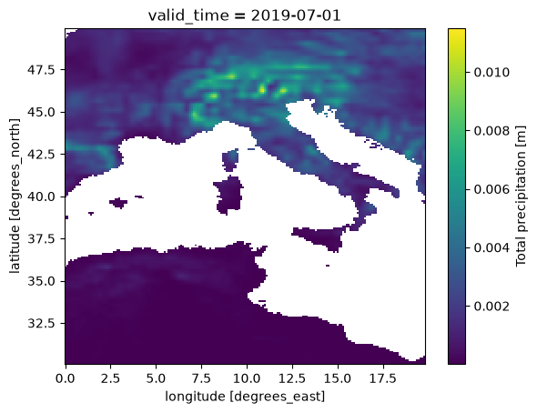
Select the time interval of interest#
We take the 30 year period from 1990 to 2019, aligned on the 10 year time chunks, and we finally have a definition of the data we want to download.
[5]:
tp_aoi_toi = tp_aoi.sel(valid_time=slice("1990", "2019"))
tp_aoi_toi
[5]:
<xarray.DataArray 'tp' (valid_time: 360, latitude: 400, longitude: 600)> Size: 346MB
dask.array<getitem, shape=(360, 400, 600), dtype=float32, chunksize=(120, 200, 200), chunktype=numpy.ndarray>
Coordinates:
  * valid_time  (valid_time) datetime64[ns] 3kB 1990-01-01 ... 2019-12-01
  * latitude    (latitude) float64 3kB 70.0 69.9 69.8 69.7 ... 30.3 30.2 30.1
  * longitude   (longitude) float64 5kB -20.0 -19.9 -19.8 ... 39.7 39.8 39.9
Attributes: (12/31)
    GRIB_paramId:                             228
    GRIB_dataType:                            fc
    GRIB_numberOfPoints:                      6483600
    GRIB_typeOfLevel:                         surface
    GRIB_stepUnits:                           1
    GRIB_gridType:                            regular_ll
    ...                                       ...
    GRIB_totalNumber:                         0
    GRIB_units:                               m
    long_name:                                Total precipitation
    units:                                    m
    standard_name:                            unknown
last_ingested_valid_time_index: 920- valid_time: 360
- latitude: 400
- longitude: 600
- dask.array<chunksize=(120, 200, 200), meta=np.ndarray>
Array Chunk Bytes 329.59 MiB 18.31 MiB Shape (360, 400, 600) (120, 200, 200) Dask graph 18 chunks in 6 graph layers Data type float32 numpy.ndarray - valid_time(valid_time)datetime64[ns]1990-01-01 ... 2019-12-01
array(['1990-01-01T00:00:00.000000000', '1990-02-01T00:00:00.000000000', '1990-03-01T00:00:00.000000000', ..., '2019-10-01T00:00:00.000000000', '2019-11-01T00:00:00.000000000', '2019-12-01T00:00:00.000000000'], shape=(360,), dtype='datetime64[ns]') - latitude(latitude)float6470.0 69.9 69.8 ... 30.3 30.2 30.1
- units :
- degrees_north
- standard_name :
- latitude
- long_name :
- latitude
- stored_direction :
- decreasing
array([70. , 69.9, 69.8, ..., 30.3, 30.2, 30.1], shape=(400,))
- longitude(longitude)float64-20.0 -19.9 -19.8 ... 39.8 39.9
- units :
- degrees_east
- standard_name :
- longitude
- long_name :
- longitude
array([-20. , -19.9, -19.8, ..., 39.7, 39.8, 39.9], shape=(600,))
- GRIB_paramId :
- 228
- GRIB_dataType :
- fc
- GRIB_numberOfPoints :
- 6483600
- GRIB_typeOfLevel :
- surface
- GRIB_stepUnits :
- 1
- GRIB_gridType :
- regular_ll
- GRIB_uvRelativeToGrid :
- 0
- GRIB_NV :
- 0
- GRIB_Nx :
- 3600
- GRIB_Ny :
- 1801
- GRIB_cfName :
- unknown
- GRIB_cfVarName :
- tp
- GRIB_gridDefinitionDescription :
- Latitude/Longitude Grid
- GRIB_iDirectionIncrementInDegrees :
- 0.1
- GRIB_iScansNegatively :
- 0
- GRIB_jDirectionIncrementInDegrees :
- 0.1
- GRIB_jPointsAreConsecutive :
- 0
- GRIB_jScansPositively :
- 0
- GRIB_latitudeOfFirstGridPointInDegrees :
- 90.0
- GRIB_latitudeOfLastGridPointInDegrees :
- -90.0
- GRIB_longitudeOfFirstGridPointInDegrees :
- 0.0
- GRIB_longitudeOfLastGridPointInDegrees :
- 359.9
- GRIB_missingValue :
- 3.4028234663852886e+38
- GRIB_name :
- Total precipitation
- GRIB_shortName :
- tp
- GRIB_totalNumber :
- 0
- GRIB_units :
- m
- long_name :
- Total precipitation
- units :
- m
- standard_name :
- unknown
- last_ingested_valid_time_index :
- 920
From the representation above we learn a few things:
the uncompressed data to be downloaded, e.g. 346MiB (compression depends on the dataset and the variable)
the number of chunks to be downloaded, e.g. 18, that is 2 latitude chunks x 3 longitude chunks x 3 time chunks
Download the data to memory#
Finally we are ready to download only the data that we are interested in, in memory.
The best practice is to call the .compute() method load the data into a numpy array in memory.
This operation is the slow one, it can take a couple of minutes.
It depends on the download speed of your internet connection and on the load on the Earth Data Hub. The closer you are to the data the faster it is, and this is one of the reason the EDH is best suited to be used from within the DestinE platform.
[6]:
%%time

tp_aoi_toi_data = tp_aoi_toi.compute()
CPU times: user 3.2 s, sys: 1.18 s, total: 4.38 s
Wall time: 1min 3s
Perform any computation#
Prepare the raw data#
In the ERA5-Land monthly averages, accumulated variables like tp hold the average daily accumulation in metres. We convert it to the monthly total in millimetres.
[7]:
days_in_month = tp_aoi_toi_data.valid_time.dt.days_in_month
tp_aoi_toi_data_mm = tp_aoi_toi_data * 1000 * days_in_month
tp_aoi_toi_data_mm.attrs["units"] = "mm"
tp_aoi_toi_data_mm.attrs["long_name"] = "monthly precipitation"
tp_aoi_toi_data_mm
[7]:
<xarray.DataArray (valid_time: 360, latitude: 400, longitude: 600)> Size: 691MB
array([[[        nan,         nan,         nan, ...,         nan,
                 nan,         nan],
        [        nan,         nan,         nan, ...,         nan,
                 nan,         nan],
        [        nan,         nan,         nan, ...,         nan,
                 nan,         nan],
        ...,
        [        nan,         nan,         nan, ...,  7.31937587,
          8.21599364,  9.1278553 ],
        [        nan,         nan,         nan, ...,  7.30459392,
          8.18550587,  9.06503201],
        [        nan,         nan,         nan, ...,  7.98410177,
          8.98650289, 10.0120008 ]],

       [[        nan,         nan,         nan, ...,         nan,
                 nan,         nan],
        [        nan,         nan,         nan, ...,         nan,
                 nan,         nan],
        [        nan,         nan,         nan, ...,         nan,
                 nan,         nan],
...
        [        nan,         nan,         nan, ...,  9.45657492,
          9.67562199,  9.8374486 ],
        [        nan,         nan,         nan, ...,  9.04887915,
          9.1329217 ,  9.19371843],
        [        nan,         nan,         nan, ...,  8.8763237 ,
          9.01848078,  9.12666321]],

       [[        nan,         nan,         nan, ...,         nan,
                 nan,         nan],
        [        nan,         nan,         nan, ...,         nan,
                 nan,         nan],
        [        nan,         nan,         nan, ...,         nan,
                 nan,         nan],
        ...,
        [        nan,         nan,         nan, ...,  4.10152972,
          4.25766408,  4.37776744],
        [        nan,         nan,         nan, ...,  3.42895091,
          3.52688134,  3.61626595],
        [        nan,         nan,         nan, ...,  3.1568706 ,
          3.1735003 ,  3.14555317]]], shape=(360, 400, 600))
Coordinates:
  * valid_time  (valid_time) datetime64[ns] 3kB 1990-01-01 ... 2019-12-01
  * latitude    (latitude) float64 3kB 70.0 69.9 69.8 69.7 ... 30.3 30.2 30.1
  * longitude   (longitude) float64 5kB -20.0 -19.9 -19.8 ... 39.7 39.8 39.9
Attributes: (12/31)
    GRIB_paramId:                             228
    GRIB_dataType:                            fc
    GRIB_numberOfPoints:                      6483600
    GRIB_typeOfLevel:                         surface
    GRIB_stepUnits:                           1
    GRIB_gridType:                            regular_ll
    ...                                       ...
    GRIB_totalNumber:                         0
    GRIB_units:                               m
    long_name:                                monthly precipitation
    units:                                    mm
    standard_name:                            unknown
last_ingested_valid_time_index: 920- valid_time: 360
- latitude: 400
- longitude: 600
- nan nan nan nan nan nan nan ... 2.256 2.591 2.92 3.157 3.174 3.146
array([[[ nan, nan, nan, ..., nan, nan, nan], [ nan, nan, nan, ..., nan, nan, nan], [ nan, nan, nan, ..., nan, nan, nan], ..., [ nan, nan, nan, ..., 7.31937587, 8.21599364, 9.1278553 ], [ nan, nan, nan, ..., 7.30459392, 8.18550587, 9.06503201], [ nan, nan, nan, ..., 7.98410177, 8.98650289, 10.0120008 ]], [[ nan, nan, nan, ..., nan, nan, nan], [ nan, nan, nan, ..., nan, nan, nan], [ nan, nan, nan, ..., nan, nan, nan], ... [ nan, nan, nan, ..., 9.45657492, 9.67562199, 9.8374486 ], [ nan, nan, nan, ..., 9.04887915, 9.1329217 , 9.19371843], [ nan, nan, nan, ..., 8.8763237 , 9.01848078, 9.12666321]], [[ nan, nan, nan, ..., nan, nan, nan], [ nan, nan, nan, ..., nan, nan, nan], [ nan, nan, nan, ..., nan, nan, nan], ..., [ nan, nan, nan, ..., 4.10152972, 4.25766408, 4.37776744], [ nan, nan, nan, ..., 3.42895091, 3.52688134, 3.61626595], [ nan, nan, nan, ..., 3.1568706 , 3.1735003 , 3.14555317]]], shape=(360, 400, 600)) - valid_time(valid_time)datetime64[ns]1990-01-01 ... 2019-12-01
array(['1990-01-01T00:00:00.000000000', '1990-02-01T00:00:00.000000000', '1990-03-01T00:00:00.000000000', ..., '2019-10-01T00:00:00.000000000', '2019-11-01T00:00:00.000000000', '2019-12-01T00:00:00.000000000'], shape=(360,), dtype='datetime64[ns]') - latitude(latitude)float6470.0 69.9 69.8 ... 30.3 30.2 30.1
- units :
- degrees_north
- standard_name :
- latitude
- long_name :
- latitude
- stored_direction :
- decreasing
array([70. , 69.9, 69.8, ..., 30.3, 30.2, 30.1], shape=(400,))
- longitude(longitude)float64-20.0 -19.9 -19.8 ... 39.8 39.9
- units :
- degrees_east
- standard_name :
- longitude
- long_name :
- longitude
array([-20. , -19.9, -19.8, ..., 39.7, 39.8, 39.9], shape=(600,))
- GRIB_paramId :
- 228
- GRIB_dataType :
- fc
- GRIB_numberOfPoints :
- 6483600
- GRIB_typeOfLevel :
- surface
- GRIB_stepUnits :
- 1
- GRIB_gridType :
- regular_ll
- GRIB_uvRelativeToGrid :
- 0
- GRIB_NV :
- 0
- GRIB_Nx :
- 3600
- GRIB_Ny :
- 1801
- GRIB_cfName :
- unknown
- GRIB_cfVarName :
- tp
- GRIB_gridDefinitionDescription :
- Latitude/Longitude Grid
- GRIB_iDirectionIncrementInDegrees :
- 0.1
- GRIB_iScansNegatively :
- 0
- GRIB_jDirectionIncrementInDegrees :
- 0.1
- GRIB_jPointsAreConsecutive :
- 0
- GRIB_jScansPositively :
- 0
- GRIB_latitudeOfFirstGridPointInDegrees :
- 90.0
- GRIB_latitudeOfLastGridPointInDegrees :
- -90.0
- GRIB_longitudeOfFirstGridPointInDegrees :
- 0.0
- GRIB_longitudeOfLastGridPointInDegrees :
- 359.9
- GRIB_missingValue :
- 3.4028234663852886e+38
- GRIB_name :
- Total precipitation
- GRIB_shortName :
- tp
- GRIB_totalNumber :
- 0
- GRIB_units :
- m
- long_name :
- monthly precipitation
- units :
- mm
- standard_name :
- unknown
- last_ingested_valid_time_index :
- 920
Annual totals#
Monthly data is convenient to describe the seasons, but the year to year variability of the climate is easier to read from annual totals.
skipna=False keeps the sea, where ERA5-Land has no data, as missing values instead of zeros.
[8]:
%%time

tp_aoi_toi_annual = tp_aoi_toi_data_mm.groupby("valid_time.year").sum(skipna=False)
tp_aoi_toi_annual.attrs["long_name"] = "annual precipitation"
tp_aoi_toi_annual
CPU times: user 79.9 ms, sys: 85.6 ms, total: 166 ms
Wall time: 168 ms
[8]:
<xarray.DataArray (year: 30, latitude: 400, longitude: 600)> Size: 58MB
array([[[         nan,          nan,          nan, ...,          nan,
                  nan,          nan],
        [         nan,          nan,          nan, ...,          nan,
                  nan,          nan],
        [         nan,          nan,          nan, ...,          nan,
                  nan,          nan],
        ...,
        [         nan,          nan,          nan, ...,  24.92439793,
          25.07522749,  25.26078897],
        [         nan,          nan,          nan, ...,  21.5028231 ,
          21.87265595,  22.23910531],
        [         nan,          nan,          nan, ...,  19.75102682,
          20.42841126,  21.15695883]],

       [[         nan,          nan,          nan, ...,          nan,
                  nan,          nan],
        [         nan,          nan,          nan, ...,          nan,
                  nan,          nan],
        [         nan,          nan,          nan, ...,          nan,
                  nan,          nan],
...
        [         nan,          nan,          nan, ..., 119.6222229 ,
         122.97250127, 126.16039609],
        [         nan,          nan,          nan, ..., 121.51340378,
         124.77888149, 127.90926342],
        [         nan,          nan,          nan, ..., 122.83895892,
         126.98248011, 130.60840761]],

       [[         nan,          nan,          nan, ...,          nan,
                  nan,          nan],
        [         nan,          nan,          nan, ...,          nan,
                  nan,          nan],
        [         nan,          nan,          nan, ...,          nan,
                  nan,          nan],
        ...,
        [         nan,          nan,          nan, ...,  77.24080462,
          77.94956345,  78.42969376],
        [         nan,          nan,          nan, ...,  81.98950667,
          81.57885302,  81.00731153],
        [         nan,          nan,          nan, ...,  80.52301261,
          81.04289178,  81.05995361]]], shape=(30, 400, 600))
Coordinates:
  * year       (year) int64 240B 1990 1991 1992 1993 ... 2016 2017 2018 2019
  * latitude   (latitude) float64 3kB 70.0 69.9 69.8 69.7 ... 30.3 30.2 30.1
  * longitude  (longitude) float64 5kB -20.0 -19.9 -19.8 ... 39.7 39.8 39.9
Attributes: (12/31)
    GRIB_paramId:                             228
    GRIB_dataType:                            fc
    GRIB_numberOfPoints:                      6483600
    GRIB_typeOfLevel:                         surface
    GRIB_stepUnits:                           1
    GRIB_gridType:                            regular_ll
    ...                                       ...
    GRIB_totalNumber:                         0
    GRIB_units:                               m
    long_name:                                annual precipitation
    units:                                    mm
    standard_name:                            unknown
last_ingested_valid_time_index: 920- year: 30
- latitude: 400
- longitude: 600
- nan nan nan nan nan nan nan ... 71.45 74.78 78.13 80.52 81.04 81.06
array([[[ nan, nan, nan, ..., nan, nan, nan], [ nan, nan, nan, ..., nan, nan, nan], [ nan, nan, nan, ..., nan, nan, nan], ..., [ nan, nan, nan, ..., 24.92439793, 25.07522749, 25.26078897], [ nan, nan, nan, ..., 21.5028231 , 21.87265595, 22.23910531], [ nan, nan, nan, ..., 19.75102682, 20.42841126, 21.15695883]], [[ nan, nan, nan, ..., nan, nan, nan], [ nan, nan, nan, ..., nan, nan, nan], [ nan, nan, nan, ..., nan, nan, nan], ... [ nan, nan, nan, ..., 119.6222229 , 122.97250127, 126.16039609], [ nan, nan, nan, ..., 121.51340378, 124.77888149, 127.90926342], [ nan, nan, nan, ..., 122.83895892, 126.98248011, 130.60840761]], [[ nan, nan, nan, ..., nan, nan, nan], [ nan, nan, nan, ..., nan, nan, nan], [ nan, nan, nan, ..., nan, nan, nan], ..., [ nan, nan, nan, ..., 77.24080462, 77.94956345, 78.42969376], [ nan, nan, nan, ..., 81.98950667, 81.57885302, 81.00731153], [ nan, nan, nan, ..., 80.52301261, 81.04289178, 81.05995361]]], shape=(30, 400, 600)) - year(year)int641990 1991 1992 ... 2017 2018 2019
array([1990, 1991, 1992, 1993, 1994, 1995, 1996, 1997, 1998, 1999, 2000, 2001, 2002, 2003, 2004, 2005, 2006, 2007, 2008, 2009, 2010, 2011, 2012, 2013, 2014, 2015, 2016, 2017, 2018, 2019]) - latitude(latitude)float6470.0 69.9 69.8 ... 30.3 30.2 30.1
- units :
- degrees_north
- standard_name :
- latitude
- long_name :
- latitude
- stored_direction :
- decreasing
array([70. , 69.9, 69.8, ..., 30.3, 30.2, 30.1], shape=(400,))
- longitude(longitude)float64-20.0 -19.9 -19.8 ... 39.8 39.9
- units :
- degrees_east
- standard_name :
- longitude
- long_name :
- longitude
array([-20. , -19.9, -19.8, ..., 39.7, 39.8, 39.9], shape=(600,))
- GRIB_paramId :
- 228
- GRIB_dataType :
- fc
- GRIB_numberOfPoints :
- 6483600
- GRIB_typeOfLevel :
- surface
- GRIB_stepUnits :
- 1
- GRIB_gridType :
- regular_ll
- GRIB_uvRelativeToGrid :
- 0
- GRIB_NV :
- 0
- GRIB_Nx :
- 3600
- GRIB_Ny :
- 1801
- GRIB_cfName :
- unknown
- GRIB_cfVarName :
- tp
- GRIB_gridDefinitionDescription :
- Latitude/Longitude Grid
- GRIB_iDirectionIncrementInDegrees :
- 0.1
- GRIB_iScansNegatively :
- 0
- GRIB_jDirectionIncrementInDegrees :
- 0.1
- GRIB_jPointsAreConsecutive :
- 0
- GRIB_jScansPositively :
- 0
- GRIB_latitudeOfFirstGridPointInDegrees :
- 90.0
- GRIB_latitudeOfLastGridPointInDegrees :
- -90.0
- GRIB_longitudeOfFirstGridPointInDegrees :
- 0.0
- GRIB_longitudeOfLastGridPointInDegrees :
- 359.9
- GRIB_missingValue :
- 3.4028234663852886e+38
- GRIB_name :
- Total precipitation
- GRIB_shortName :
- tp
- GRIB_totalNumber :
- 0
- GRIB_units :
- m
- long_name :
- annual precipitation
- units :
- mm
- standard_name :
- unknown
- last_ingested_valid_time_index :
- 920
Mean annual precipitation#
The 30 year mean shows the wet Atlantic coasts and mountain ranges and the dry south.
[9]:
tp_aoi_toi_mean = tp_aoi_toi_annual.mean("year")
tp_aoi_toi_mean.plot(cmap="YlGnBu", vmax=2000, figsize=(7, 4))
[9]:
<matplotlib.collections.QuadMesh at 0x127667390>
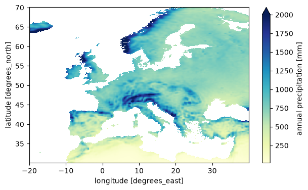
Precipitation trend#
Averaging over the whole area gives a single time series for Europe and a linear fit on it summarises the change over the period.
The simple mean over all grid points gives more weight to the high latitudes, where the grid cells are smaller; a proper area weighting would use cos(latitude) as weight, but for this example the simple mean is good enough.
Precipitation varies a lot from year to year, so the trend of a single 30 year period is uncertain.
[10]:
tp_europe_annual = tp_aoi_toi_annual.mean(["latitude", "longitude"])

tp_europe_trend = tp_europe_annual.polyfit("year", 1)
tp_europe_trend = tp_europe_trend.polyfit_coefficients.sel(degree=1)

print(f"Europe mean precipitation trend: {10 * float(tp_europe_trend):.0f} mm/decade")
Europe mean precipitation trend: 7 mm/decade
[11]:
tp_europe_annual.plot(marker="o", figsize=(8, 3))
[11]:
[<matplotlib.lines.Line2D at 0x127a05010>]
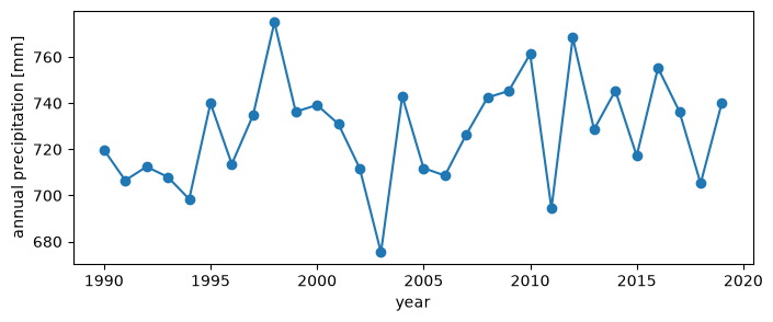
Trend map#
The same linear fit applied at every grid point, divided by the mean annual precipitation, gives the trend in percent per decade, that can be compared between wet and dry regions. Over the deserts in the south of the area the mean is close to zero and the relative trend is not meaningful.
[12]:
%%time

tp_aoi_toi_trend = tp_aoi_toi_annual.polyfit("year", 1)
tp_aoi_toi_trend = tp_aoi_toi_trend.polyfit_coefficients.sel(degree=1) * 10
tp_aoi_toi_trend = 100 * tp_aoi_toi_trend / tp_aoi_toi_mean
tp_aoi_toi_trend.attrs["units"] = "%/decade"
tp_aoi_toi_trend.attrs["long_name"] = "precipitation trend"
tp_aoi_toi_trend.plot(cmap="BrBG", vmin=-20, vmax=20, figsize=(7, 4))
CPU times: user 336 ms, sys: 18.6 ms, total: 354 ms
Wall time: 349 ms
[12]:
<matplotlib.collections.QuadMesh at 0x127a9c050>
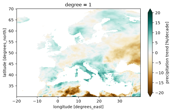
Next steps#
replace
tpwith any other variable of the dataset, e.g. the 2 metre temperaturet2mor the volumetric soil waterswvl1,replace the area and the period of interest with the ones you need, keeping in mind that the data is downloaded in chunks of 10 years x 20° x 20°.