Note
To run this notebook locally, follow the setup instructions in the GitHub repository.
Getting started with the Earth Data Hub#
This notebook reproduces the Getting Started page of the Earth Data Hub.
Earth Data Hub offers an innovative and super-efficient way to access data. Here is what you need to know to start working.
Datasets are published as Zarr stores and every user has a monthly quota of 500,000 allowed requests, so downloads must be authenticated. See the Quota & API keys page to check current consumption.
We will show how to obtain and use your authentication credentials later, let’s start by connecting to a test dataset that doesn’t need authentication.
Setup the environment#
If you are using the suggested way to run the notebook via uv run jupyter lab you are good to go. In other cases you may need to install the following Python packages:
xarray,zarr(version 3 or later),daskandaiohttpto access the datajupyterlabandmatplotlibto run the notebook and plot the data
Open your first dataset (without authentication)#
The easiest way to get started with Earth Data Hub is by using Python and Xarray, on our public test dataset.
[1]:
import xarray as xr
[2]:
test_dataset_public = xr.open_dataset(
    "https://data.earthdatahub.destine.eu/public/test-dataset-v1.zarr",
    chunks={},
    engine="zarr",
)
test_dataset_public
[2]:
<xarray.Dataset> Size: 4GB
Dimensions:               (latitude: 720, longitude: 1440,
                           age_band_lower_bound: 14, year: 71)
Coordinates:
  * latitude              (latitude) float64 6kB 90.0 89.75 ... -89.5 -89.75
  * longitude             (longitude) float64 12kB 0.0 0.25 0.5 ... 359.5 359.8
  * age_band_lower_bound  (age_band_lower_bound) int64 112B 0 5 10 ... 55 60 65
  * year                  (year) int64 568B 1950 1951 1952 ... 2018 2019 2020
Data variables:
demographic_totals (latitude, longitude, age_band_lower_bound, year) float32 4GB dask.array<chunksize=(180, 180, 14, 2), meta=np.ndarray>- latitude: 720
- longitude: 1440
- age_band_lower_bound: 14
- year: 71
- latitude(latitude)float6490.0 89.75 89.5 ... -89.5 -89.75
array([ 90. , 89.75, 89.5 , ..., -89.25, -89.5 , -89.75], shape=(720,))
- longitude(longitude)float640.0 0.25 0.5 ... 359.2 359.5 359.8
array([0.0000e+00, 2.5000e-01, 5.0000e-01, ..., 3.5925e+02, 3.5950e+02, 3.5975e+02], shape=(1440,)) - age_band_lower_bound(age_band_lower_bound)int640 5 10 15 20 25 ... 45 50 55 60 65
array([ 0, 5, 10, 15, 20, 25, 30, 35, 40, 45, 50, 55, 60, 65])
- year(year)int641950 1951 1952 ... 2018 2019 2020
array([1950, 1951, 1952, 1953, 1954, 1955, 1956, 1957, 1958, 1959, 1960, 1961,
       1962, 1963, 1964, 1965, 1966, 1967, 1968, 1969, 1970, 1971, 1972, 1973,
       1974, 1975, 1976, 1977, 1978, 1979, 1980, 1981, 1982, 1983, 1984, 1985,
       1986, 1987, 1988, 1989, 1990, 1991, 1992, 1993, 1994, 1995, 1996, 1997,
       1998, 1999, 2000, 2001, 2002, 2003, 2004, 2005, 2006, 2007, 2008, 2009,
       2010, 2011, 2012, 2013, 2014, 2015, 2016, 2017, 2018, 2019, 2020])
- demographic_totals(latitude, longitude, age_band_lower_bound, year)float32dask.array<chunksize=(180, 180, 14, 2), meta=np.ndarray>
- last_ingested_year_index :
- 70
Array Chunk Bytes 3.84 GiB 3.46 MiB Shape (720, 1440, 14, 71) (180, 180, 14, 2) Dask graph 1152 chunks in 2 graph layers Data type float32 numpy.ndarray
We can process and plot a portion of the data in a few lines of code.
[3]:
demographic_totals_2020 = test_dataset_public["demographic_totals"].sel(year=2020)

world_population_2020 = demographic_totals_2020.sum("age_band_lower_bound")

world_population_2020.plot(vmax=500_000)
[3]:
<matplotlib.collections.QuadMesh at 0x115dc5550>
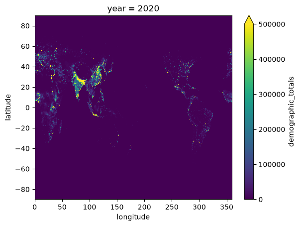
Note that we performed several operations:
selection: we choose the variable
demographic_totalsand the year2020aggregation: we summed over all the age classes
display: we plotted the data with simple configuration options
Setup your credentials for authenticated data access#
To access most datasets on Earth Data Hub you simply need to obtain an API key and instruct your tools to use it when downloading the data.
How to obtain an Earth Data Hub API key#
Register an account on the DestinE Platform.
Visit the Quota & API keys page.
Copy your default API key (or generate a new one).
Now we are ready to access the same small test dataset, but this time from a URL that is authorization protected: https://data.earthdatahub.destine.eu/private/test-dataset-v1.zarr.
Adding the API key to the URL#
The easiest way is to pass the API key as a password in the Zarr store URL, for example:
[4]:
import os

edh_key = os.getenv("EDH_KEY", "<write your API key here>")

assert edh_key.startswith("edh_key_"), (
    f"Your API key is a long string starting with 'edh_key_', not {edh_key!r}"
)
[5]:
test_dataset_url = xr.open_dataset(
    f"https://edh:{edh_key}@data.earthdatahub.destine.eu/private/test-dataset-v1.zarr",
    chunks={},
    engine="zarr",
)
test_dataset_url
[5]:
<xarray.Dataset> Size: 4GB
Dimensions:               (latitude: 720, longitude: 1440,
                           age_band_lower_bound: 14, year: 71)
Coordinates:
  * latitude              (latitude) float64 6kB 90.0 89.75 ... -89.5 -89.75
  * longitude             (longitude) float64 12kB 0.0 0.25 0.5 ... 359.5 359.8
  * age_band_lower_bound  (age_band_lower_bound) int64 112B 0 5 10 ... 55 60 65
  * year                  (year) int64 568B 1950 1951 1952 ... 2018 2019 2020
Data variables:
demographic_totals (latitude, longitude, age_band_lower_bound, year) float32 4GB dask.array<chunksize=(180, 180, 14, 2), meta=np.ndarray>- latitude: 720
- longitude: 1440
- age_band_lower_bound: 14
- year: 71
- latitude(latitude)float6490.0 89.75 89.5 ... -89.5 -89.75
array([ 90. , 89.75, 89.5 , ..., -89.25, -89.5 , -89.75], shape=(720,))
- longitude(longitude)float640.0 0.25 0.5 ... 359.2 359.5 359.8
array([0.0000e+00, 2.5000e-01, 5.0000e-01, ..., 3.5925e+02, 3.5950e+02, 3.5975e+02], shape=(1440,)) - age_band_lower_bound(age_band_lower_bound)int640 5 10 15 20 25 ... 45 50 55 60 65
array([ 0, 5, 10, 15, 20, 25, 30, 35, 40, 45, 50, 55, 60, 65])
- year(year)int641950 1951 1952 ... 2018 2019 2020
array([1950, 1951, 1952, 1953, 1954, 1955, 1956, 1957, 1958, 1959, 1960, 1961,
       1962, 1963, 1964, 1965, 1966, 1967, 1968, 1969, 1970, 1971, 1972, 1973,
       1974, 1975, 1976, 1977, 1978, 1979, 1980, 1981, 1982, 1983, 1984, 1985,
       1986, 1987, 1988, 1989, 1990, 1991, 1992, 1993, 1994, 1995, 1996, 1997,
       1998, 1999, 2000, 2001, 2002, 2003, 2004, 2005, 2006, 2007, 2008, 2009,
       2010, 2011, 2012, 2013, 2014, 2015, 2016, 2017, 2018, 2019, 2020])
- demographic_totals(latitude, longitude, age_band_lower_bound, year)float32dask.array<chunksize=(180, 180, 14, 2), meta=np.ndarray>
- last_ingested_year_index :
- 70
Array Chunk Bytes 3.84 GiB 3.46 MiB Shape (720, 1440, 14, 71) (180, 180, 14, 2) Dask graph 1152 chunks in 2 graph layers Data type float32 numpy.ndarray
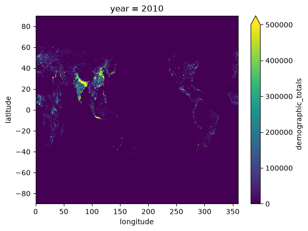
We can now test plotting the private dataset.
[6]:
demographic_totals_2010 = test_dataset_url["demographic_totals"].sel(year=2010)

world_population_2010 = demographic_totals_2010.sum("age_band_lower_bound")

world_population_2010.plot(vmax=500_000)
[6]:
<matplotlib.collections.QuadMesh at 0x1179974d0>
Configuring the API key in the netrc file#
A more convenient way to set up the API key if you plan to use the system, is to configure the netrc file (~/.netrc on Linux and MacOS, C:\Users\<username>\_netrc on Windows) as follows:
machine data.earthdatahub.destine.eu
  password <write your API key here>

machine api.earthdatahub.destine.eu
  password <write your API key here>
Earth Data Hub has two data access entry points, so the file needs an entry for each one. You can also retrieve your netrc file directly from the Quota & API keys page using the ⓘ button.
Once this is set up you can use the URL above directly and similarly, the other URL that you find in the catalogue:
[7]:
test_dataset_netrc = xr.open_dataset(
    "https://data.earthdatahub.destine.eu/private/test-dataset-v1.zarr",
    storage_options={"client_kwargs": {"trust_env": True}},
    chunks={},
    engine="zarr",
)
test_dataset_netrc
[7]:
<xarray.Dataset> Size: 4GB
Dimensions:               (latitude: 720, longitude: 1440,
                           age_band_lower_bound: 14, year: 71)
Coordinates:
  * latitude              (latitude) float64 6kB 90.0 89.75 ... -89.5 -89.75
  * longitude             (longitude) float64 12kB 0.0 0.25 0.5 ... 359.5 359.8
  * age_band_lower_bound  (age_band_lower_bound) int64 112B 0 5 10 ... 55 60 65
  * year                  (year) int64 568B 1950 1951 1952 ... 2018 2019 2020
Data variables:
demographic_totals (latitude, longitude, age_band_lower_bound, year) float32 4GB dask.array<chunksize=(180, 180, 14, 2), meta=np.ndarray>- latitude: 720
- longitude: 1440
- age_band_lower_bound: 14
- year: 71
- latitude(latitude)float6490.0 89.75 89.5 ... -89.5 -89.75
array([ 90. , 89.75, 89.5 , ..., -89.25, -89.5 , -89.75], shape=(720,))
- longitude(longitude)float640.0 0.25 0.5 ... 359.2 359.5 359.8
array([0.0000e+00, 2.5000e-01, 5.0000e-01, ..., 3.5925e+02, 3.5950e+02, 3.5975e+02], shape=(1440,)) - age_band_lower_bound(age_band_lower_bound)int640 5 10 15 20 25 ... 45 50 55 60 65
array([ 0, 5, 10, 15, 20, 25, 30, 35, 40, 45, 50, 55, 60, 65])
- year(year)int641950 1951 1952 ... 2018 2019 2020
array([1950, 1951, 1952, 1953, 1954, 1955, 1956, 1957, 1958, 1959, 1960, 1961,
       1962, 1963, 1964, 1965, 1966, 1967, 1968, 1969, 1970, 1971, 1972, 1973,
       1974, 1975, 1976, 1977, 1978, 1979, 1980, 1981, 1982, 1983, 1984, 1985,
       1986, 1987, 1988, 1989, 1990, 1991, 1992, 1993, 1994, 1995, 1996, 1997,
       1998, 1999, 2000, 2001, 2002, 2003, 2004, 2005, 2006, 2007, 2008, 2009,
       2010, 2011, 2012, 2013, 2014, 2015, 2016, 2017, 2018, 2019, 2020])
- demographic_totals(latitude, longitude, age_band_lower_bound, year)float32dask.array<chunksize=(180, 180, 14, 2), meta=np.ndarray>
- last_ingested_year_index :
- 70
Array Chunk Bytes 3.84 GiB 3.46 MiB Shape (720, 1440, 14, 71) (180, 180, 14, 2) Dask graph 1152 chunks in 2 graph layers Data type float32 numpy.ndarray
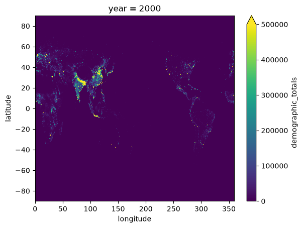
And we are ready to test plotting on the private dataset.
[8]:
demographic_totals_2000 = test_dataset_netrc["demographic_totals"].sel(year=2000)

world_population_2000 = demographic_totals_2000.sum("age_band_lower_bound")

world_population_2000.plot(vmax=500_000)
[8]:
<matplotlib.collections.QuadMesh at 0x117b3b9d0>
Keep in mind that some tools do not use the netrc file by default, but can be instructed to do so, for example, the storage_options={"client_kwargs":{"trust_env":True}} option is needed by Xarray / Zarr.
Access your first real dataset#
How to use the catalogue#
Datasets are offered in the Earth Data Hub catalogue as Zarr stores, even if a dataset is identified by a single URL its size may be very large, easily hundreds of terabytes.
You will find the code snippet to access the data with Xarray on the dataset page and that will work out of the box after you set up the netrc file as described above.
Be careful, do not try to download an entire dataset, chances are that you will exceed your quota well before you come even close! Instead, we show how to access and work with large datasets in our tutorials.
ERA5 monthly averages from 1940 to present#
A good dataset to start with is ERA5 monthly averaged data on single levels: every variable is about 4GiB in size, small compared to the 2.9TiB of an hourly ERA5 variable, and it is relatively easy to handle.
If you managed to set up your netrc file you can just copy the code snippet in the dataset page:
[9]:
era5_monthly = xr.open_dataset(
    "https://data.earthdatahub.destine.eu/era5/era5-single-levels-atmosphere-monthly-v0.zarr",
    storage_options={"client_kwargs": {"trust_env": True}},
    chunks={},
    engine="zarr",
)
era5_monthly
[9]:
<xarray.Dataset> Size: 860GB
Dimensions:         (valid_time: 1041, latitude: 721, longitude: 1440)
Coordinates:
  * valid_time      (valid_time) datetime64[ns] 8kB 1940-01-01 ... 2026-09-01
  * latitude        (latitude) float64 6kB 90.0 89.75 89.5 ... -89.75 -90.0
  * longitude       (longitude) float64 12kB 0.0 0.25 0.5 ... 359.2 359.5 359.8
Data variables: (12/213)
    alnid           (valid_time, latitude, longitude) float32 4GB dask.array<chunksize=(120, 240, 240), meta=np.ndarray>
    alnip           (valid_time, latitude, longitude) float32 4GB dask.array<chunksize=(120, 240, 240), meta=np.ndarray>
    aluvd           (valid_time, latitude, longitude) float32 4GB dask.array<chunksize=(120, 240, 240), meta=np.ndarray>
    aluvp           (valid_time, latitude, longitude) float32 4GB dask.array<chunksize=(120, 240, 240), meta=np.ndarray>
    anor            (latitude, longitude) float32 4MB dask.array<chunksize=(240, 240), meta=np.ndarray>
    asn             (valid_time, latitude, longitude) float32 4GB dask.array<chunksize=(120, 240, 240), meta=np.ndarray>
    ...              ...
    vithen          (valid_time, latitude, longitude) float32 4GB dask.array<chunksize=(120, 240, 240), meta=np.ndarray>
    vitoe           (valid_time, latitude, longitude) float32 4GB dask.array<chunksize=(120, 240, 240), meta=np.ndarray>
    viwve           (valid_time, latitude, longitude) float32 4GB dask.array<chunksize=(120, 240, 240), meta=np.ndarray>
    viwvn           (valid_time, latitude, longitude) float32 4GB dask.array<chunksize=(120, 240, 240), meta=np.ndarray>
    z               (latitude, longitude) float32 4MB dask.array<chunksize=(240, 240), meta=np.ndarray>
    zust            (valid_time, latitude, longitude) float32 4GB dask.array<chunksize=(120, 240, 240), meta=np.ndarray>
Attributes:
    GRIB_edition:            1
    GRIB_centre:             ecmf
    GRIB_centreDescription:  European Centre for Medium-Range Weather Forecasts
    GRIB_subCentre:          0
    Conventions:             CF-1.7
    institution:             European Centre for Medium-Range Weather Forecasts
history: 2026-10-08T14:35 GRIB to CDM+CF via cfgrib-0.9.1...- valid_time: 1041
- latitude: 721
- longitude: 1440
- valid_time(valid_time)datetime64[ns]1940-01-01 ... 2026-09-01
array(['1940-01-01T00:00:00.000000000', '1940-02-01T00:00:00.000000000', '1940-03-01T00:00:00.000000000', ..., '2026-07-01T00:00:00.000000000', '2026-08-01T00:00:00.000000000', '2026-09-01T00:00:00.000000000'], shape=(1041,), dtype='datetime64[ns]') - latitude(latitude)float6490.0 89.75 89.5 ... -89.75 -90.0
- units :
- degrees_north
- standard_name :
- latitude
- long_name :
- latitude
- stored_direction :
- decreasing
array([ 90. , 89.75, 89.5 , ..., -89.5 , -89.75, -90. ], shape=(721,))
- longitude(longitude)float640.0 0.25 0.5 ... 359.2 359.5 359.8
- units :
- degrees_east
- standard_name :
- longitude
- long_name :
- longitude
array([0.0000e+00, 2.5000e-01, 5.0000e-01, ..., 3.5925e+02, 3.5950e+02,
       3.5975e+02], shape=(1440,))
- alnid(valid_time, latitude, longitude)float32dask.array<chunksize=(120, 240, 240), meta=np.ndarray>
- GRIB_paramId :
- 18
- GRIB_dataType :
- an
- GRIB_numberOfPoints :
- 1038240
- GRIB_typeOfLevel :
- surface
- GRIB_stepUnits :
- 1
- GRIB_stepType :
- avgua
- GRIB_gridType :
- regular_ll
- GRIB_uvRelativeToGrid :
- 0
- GRIB_NV :
- 0
- GRIB_Nx :
- 1440
- GRIB_Ny :
- 721
- GRIB_cfName :
- unknown
- GRIB_cfVarName :
- alnid
- GRIB_gridDefinitionDescription :
- Latitude/Longitude Grid
- GRIB_iDirectionIncrementInDegrees :
- 0.25
- GRIB_iScansNegatively :
- 0
- GRIB_jDirectionIncrementInDegrees :
- 0.25
- GRIB_jPointsAreConsecutive :
- 0
- GRIB_jScansPositively :
- 0
- GRIB_latitudeOfFirstGridPointInDegrees :
- 90.0
- GRIB_latitudeOfLastGridPointInDegrees :
- -90.0
- GRIB_longitudeOfFirstGridPointInDegrees :
- 0.0
- GRIB_longitudeOfLastGridPointInDegrees :
- 359.75
- GRIB_missingValue :
- 3.4028234663852886e+38
- GRIB_name :
- Near IR albedo for diffuse radiation (climatological)
- GRIB_shortName :
- alnid
- GRIB_totalNumber :
- 0
- GRIB_units :
- (0 - 1)
- long_name :
- Near IR albedo for diffuse radiation (climatological)
- units :
- (0 - 1)
- standard_name :
- unknown
- last_ingested_valid_time_index :
- 1040
Array Chunk Bytes 4.03 GiB 26.37 MiB Shape (1041, 721, 1440) (120, 240, 240) Dask graph 216 chunks in 2 graph layers Data type float32 numpy.ndarray - alnip(valid_time, latitude, longitude)float32dask.array<chunksize=(120, 240, 240), meta=np.ndarray>
- GRIB_paramId :
- 17
- GRIB_dataType :
- an
- GRIB_numberOfPoints :
- 1038240
- GRIB_typeOfLevel :
- surface
- GRIB_stepUnits :
- 1
- GRIB_stepType :
- avgua
- GRIB_gridType :
- regular_ll
- GRIB_uvRelativeToGrid :
- 0
- GRIB_NV :
- 0
- GRIB_Nx :
- 1440
- GRIB_Ny :
- 721
- GRIB_cfName :
- unknown
- GRIB_cfVarName :
- alnip
- GRIB_gridDefinitionDescription :
- Latitude/Longitude Grid
- GRIB_iDirectionIncrementInDegrees :
- 0.25
- GRIB_iScansNegatively :
- 0
- GRIB_jDirectionIncrementInDegrees :
- 0.25
- GRIB_jPointsAreConsecutive :
- 0
- GRIB_jScansPositively :
- 0
- GRIB_latitudeOfFirstGridPointInDegrees :
- 90.0
- GRIB_latitudeOfLastGridPointInDegrees :
- -90.0
- GRIB_longitudeOfFirstGridPointInDegrees :
- 0.0
- GRIB_longitudeOfLastGridPointInDegrees :
- 359.75
- GRIB_missingValue :
- 3.4028234663852886e+38
- GRIB_name :
- Near IR albedo for direct radiation (climatological)
- GRIB_shortName :
- alnip
- GRIB_totalNumber :
- 0
- GRIB_units :
- (0 - 1)
- long_name :
- Near IR albedo for direct radiation (climatological)
- units :
- (0 - 1)
- standard_name :
- unknown
- last_ingested_valid_time_index :
- 1040
Array Chunk Bytes 4.03 GiB 26.37 MiB Shape (1041, 721, 1440) (120, 240, 240) Dask graph 216 chunks in 2 graph layers Data type float32 numpy.ndarray - aluvd(valid_time, latitude, longitude)float32dask.array<chunksize=(120, 240, 240), meta=np.ndarray>
- GRIB_paramId :
- 16
- GRIB_dataType :
- an
- GRIB_numberOfPoints :
- 1038240
- GRIB_typeOfLevel :
- surface
- GRIB_stepUnits :
- 1
- GRIB_stepType :
- avgua
- GRIB_gridType :
- regular_ll
- GRIB_uvRelativeToGrid :
- 0
- GRIB_NV :
- 0
- GRIB_Nx :
- 1440
- GRIB_Ny :
- 721
- GRIB_cfName :
- unknown
- GRIB_cfVarName :
- aluvd
- GRIB_gridDefinitionDescription :
- Latitude/Longitude Grid
- GRIB_iDirectionIncrementInDegrees :
- 0.25
- GRIB_iScansNegatively :
- 0
- GRIB_jDirectionIncrementInDegrees :
- 0.25
- GRIB_jPointsAreConsecutive :
- 0
- GRIB_jScansPositively :
- 0
- GRIB_latitudeOfFirstGridPointInDegrees :
- 90.0
- GRIB_latitudeOfLastGridPointInDegrees :
- -90.0
- GRIB_longitudeOfFirstGridPointInDegrees :
- 0.0
- GRIB_longitudeOfLastGridPointInDegrees :
- 359.75
- GRIB_missingValue :
- 3.4028234663852886e+38
- GRIB_name :
- UV visible albedo for diffuse radiation (climatological)
- GRIB_shortName :
- aluvd
- GRIB_totalNumber :
- 0
- GRIB_units :
- (0 - 1)
- long_name :
- UV visible albedo for diffuse radiation (climatological)
- units :
- (0 - 1)
- standard_name :
- unknown
- last_ingested_valid_time_index :
- 1040
Array Chunk Bytes 4.03 GiB 26.37 MiB Shape (1041, 721, 1440) (120, 240, 240) Dask graph 216 chunks in 2 graph layers Data type float32 numpy.ndarray - aluvp(valid_time, latitude, longitude)float32dask.array<chunksize=(120, 240, 240), meta=np.ndarray>
- GRIB_paramId :
- 15
- GRIB_dataType :
- an
- GRIB_numberOfPoints :
- 1038240
- GRIB_typeOfLevel :
- surface
- GRIB_stepUnits :
- 1
- GRIB_stepType :
- avgua
- GRIB_gridType :
- regular_ll
- GRIB_uvRelativeToGrid :
- 0
- GRIB_NV :
- 0
- GRIB_Nx :
- 1440
- GRIB_Ny :
- 721
- GRIB_cfName :
- unknown
- GRIB_cfVarName :
- aluvp
- GRIB_gridDefinitionDescription :
- Latitude/Longitude Grid
- GRIB_iDirectionIncrementInDegrees :
- 0.25
- GRIB_iScansNegatively :
- 0
- GRIB_jDirectionIncrementInDegrees :
- 0.25
- GRIB_jPointsAreConsecutive :
- 0
- GRIB_jScansPositively :
- 0
- GRIB_latitudeOfFirstGridPointInDegrees :
- 90.0
- GRIB_latitudeOfLastGridPointInDegrees :
- -90.0
- GRIB_longitudeOfFirstGridPointInDegrees :
- 0.0
- GRIB_longitudeOfLastGridPointInDegrees :
- 359.75
- GRIB_missingValue :
- 3.4028234663852886e+38
- GRIB_name :
- UV visible albedo for direct radiation (climatological)
- GRIB_shortName :
- aluvp
- GRIB_totalNumber :
- 0
- GRIB_units :
- (0 - 1)
- long_name :
- UV visible albedo for direct radiation (climatological)
- units :
- (0 - 1)
- standard_name :
- unknown
- last_ingested_valid_time_index :
- 1040
Array Chunk Bytes 4.03 GiB 26.37 MiB Shape (1041, 721, 1440) (120, 240, 240) Dask graph 216 chunks in 2 graph layers Data type float32 numpy.ndarray - anor(latitude, longitude)float32dask.array<chunksize=(240, 240), meta=np.ndarray>
- GRIB_paramId :
- 162
- GRIB_dataType :
- an
- GRIB_numberOfPoints :
- 1038240
- GRIB_typeOfLevel :
- surface
- GRIB_stepUnits :
- 1
- GRIB_stepType :
- avgua
- GRIB_gridType :
- regular_ll
- GRIB_uvRelativeToGrid :
- 0
- GRIB_NV :
- 0
- GRIB_Nx :
- 1440
- GRIB_Ny :
- 721
- GRIB_cfName :
- unknown
- GRIB_cfVarName :
- anor
- GRIB_gridDefinitionDescription :
- Latitude/Longitude Grid
- GRIB_iDirectionIncrementInDegrees :
- 0.25
- GRIB_iScansNegatively :
- 0
- GRIB_jDirectionIncrementInDegrees :
- 0.25
- GRIB_jPointsAreConsecutive :
- 0
- GRIB_jScansPositively :
- 0
- GRIB_latitudeOfFirstGridPointInDegrees :
- 90.0
- GRIB_latitudeOfLastGridPointInDegrees :
- -90.0
- GRIB_longitudeOfFirstGridPointInDegrees :
- 0.0
- GRIB_longitudeOfLastGridPointInDegrees :
- 359.75
- GRIB_missingValue :
- 3.4028234663852886e+38
- GRIB_name :
- Angle of sub-gridscale orography
- GRIB_shortName :
- anor
- GRIB_totalNumber :
- 0
- GRIB_units :
- radians
- long_name :
- Angle of sub-gridscale orography
- units :
- radians
- standard_name :
- unknown
- last_ingested_latitude_index :
- 720
Array Chunk Bytes 3.96 MiB 225.00 kiB Shape (721, 1440) (240, 240) Dask graph 24 chunks in 2 graph layers Data type float32 numpy.ndarray - asn(valid_time, latitude, longitude)float32dask.array<chunksize=(120, 240, 240), meta=np.ndarray>
- GRIB_paramId :
- 32
- GRIB_dataType :
- an
- GRIB_numberOfPoints :
- 1038240
- GRIB_typeOfLevel :
- surface
- GRIB_stepUnits :
- 1
- GRIB_stepType :
- avgua
- GRIB_gridType :
- regular_ll
- GRIB_uvRelativeToGrid :
- 0
- GRIB_NV :
- 0
- GRIB_Nx :
- 1440
- GRIB_Ny :
- 721
- GRIB_cfName :
- unknown
- GRIB_cfVarName :
- asn
- GRIB_gridDefinitionDescription :
- Latitude/Longitude Grid
- GRIB_iDirectionIncrementInDegrees :
- 0.25
- GRIB_iScansNegatively :
- 0
- GRIB_jDirectionIncrementInDegrees :
- 0.25
- GRIB_jPointsAreConsecutive :
- 0
- GRIB_jScansPositively :
- 0
- GRIB_latitudeOfFirstGridPointInDegrees :
- 90.0
- GRIB_latitudeOfLastGridPointInDegrees :
- -90.0
- GRIB_longitudeOfFirstGridPointInDegrees :
- 0.0
- GRIB_longitudeOfLastGridPointInDegrees :
- 359.75
- GRIB_missingValue :
- 3.4028234663852886e+38
- GRIB_name :
- Snow albedo
- GRIB_shortName :
- asn
- GRIB_totalNumber :
- 0
- GRIB_units :
- (0 - 1)
- long_name :
- Snow albedo
- units :
- (0 - 1)
- standard_name :
- unknown
- last_ingested_valid_time_index :
- 1040
Array Chunk Bytes 4.03 GiB 26.37 MiB Shape (1041, 721, 1440) (120, 240, 240) Dask graph 216 chunks in 2 graph layers Data type float32 numpy.ndarray - avg_cpr(valid_time, latitude, longitude)float32dask.array<chunksize=(120, 240, 240), meta=np.ndarray>
- GRIB_paramId :
- 235030
- GRIB_dataType :
- fc
- GRIB_numberOfPoints :
- 1038240
- GRIB_typeOfLevel :
- surface
- GRIB_stepUnits :
- 1
- GRIB_stepType :
- avgad
- GRIB_gridType :
- regular_ll
- GRIB_uvRelativeToGrid :
- 0
- GRIB_NV :
- 0
- GRIB_Nx :
- 1440
- GRIB_Ny :
- 721
- GRIB_cfName :
- unknown
- GRIB_cfVarName :
- avg_cpr
- GRIB_gridDefinitionDescription :
- Latitude/Longitude Grid
- GRIB_iDirectionIncrementInDegrees :
- 0.25
- GRIB_iScansNegatively :
- 0
- GRIB_jDirectionIncrementInDegrees :
- 0.25
- GRIB_jPointsAreConsecutive :
- 0
- GRIB_jScansPositively :
- 0
- GRIB_latitudeOfFirstGridPointInDegrees :
- 90.0
- GRIB_latitudeOfLastGridPointInDegrees :
- -90.0
- GRIB_longitudeOfFirstGridPointInDegrees :
- 0.0
- GRIB_longitudeOfLastGridPointInDegrees :
- 359.75
- GRIB_missingValue :
- 3.4028234663852886e+38
- GRIB_name :
- Time-mean convective precipitation rate
- GRIB_shortName :
- avg_cpr
- GRIB_totalNumber :
- 0
- GRIB_units :
- kg m**-2 s**-1
- long_name :
- Time-mean convective precipitation rate
- units :
- kg m**-2 s**-1
- standard_name :
- unknown
- last_ingested_valid_time_index :
- 1040
Array Chunk Bytes 4.03 GiB 26.37 MiB Shape (1041, 721, 1440) (120, 240, 240) Dask graph 216 chunks in 2 graph layers Data type float32 numpy.ndarray - avg_csfr(valid_time, latitude, longitude)float32dask.array<chunksize=(120, 240, 240), meta=np.ndarray>
- GRIB_paramId :
- 235056
- GRIB_dataType :
- fc
- GRIB_numberOfPoints :
- 1038240
- GRIB_typeOfLevel :
- surface
- GRIB_stepUnits :
- 1
- GRIB_stepType :
- avgad
- GRIB_gridType :
- regular_ll
- GRIB_uvRelativeToGrid :
- 0
- GRIB_NV :
- 0
- GRIB_Nx :
- 1440
- GRIB_Ny :
- 721
- GRIB_cfName :
- unknown
- GRIB_cfVarName :
- avg_csfr
- GRIB_gridDefinitionDescription :
- Latitude/Longitude Grid
- GRIB_iDirectionIncrementInDegrees :
- 0.25
- GRIB_iScansNegatively :
- 0
- GRIB_jDirectionIncrementInDegrees :
- 0.25
- GRIB_jPointsAreConsecutive :
- 0
- GRIB_jScansPositively :
- 0
- GRIB_latitudeOfFirstGridPointInDegrees :
- 90.0
- GRIB_latitudeOfLastGridPointInDegrees :
- -90.0
- GRIB_longitudeOfFirstGridPointInDegrees :
- 0.0
- GRIB_longitudeOfLastGridPointInDegrees :
- 359.75
- GRIB_missingValue :
- 3.4028234663852886e+38
- GRIB_name :
- Time-mean convective snowfall rate water equivalent
- GRIB_shortName :
- avg_csfr
- GRIB_totalNumber :
- 0
- GRIB_units :
- kg m**-2 s**-1
- long_name :
- Time-mean convective snowfall rate water equivalent
- units :
- kg m**-2 s**-1
- standard_name :
- unknown
- last_ingested_valid_time_index :
- 1040
Array Chunk Bytes 4.03 GiB 26.37 MiB Shape (1041, 721, 1440) (120, 240, 240) Dask graph 216 chunks in 2 graph layers Data type float32 numpy.ndarray - avg_esrwe(valid_time, latitude, longitude)float32dask.array<chunksize=(120, 240, 240), meta=np.ndarray>
- GRIB_paramId :
- 235023
- GRIB_dataType :
- fc
- GRIB_numberOfPoints :
- 1038240
- GRIB_typeOfLevel :
- surface
- GRIB_stepUnits :
- 1
- GRIB_stepType :
- avgad
- GRIB_gridType :
- regular_ll
- GRIB_uvRelativeToGrid :
- 0
- GRIB_NV :
- 0
- GRIB_Nx :
- 1440
- GRIB_Ny :
- 721
- GRIB_cfName :
- unknown
- GRIB_cfVarName :
- avg_esrwe
- GRIB_gridDefinitionDescription :
- Latitude/Longitude Grid
- GRIB_iDirectionIncrementInDegrees :
- 0.25
- GRIB_iScansNegatively :
- 0
- GRIB_jDirectionIncrementInDegrees :
- 0.25
- GRIB_jPointsAreConsecutive :
- 0
- GRIB_jScansPositively :
- 0
- GRIB_latitudeOfFirstGridPointInDegrees :
- 90.0
- GRIB_latitudeOfLastGridPointInDegrees :
- -90.0
- GRIB_longitudeOfFirstGridPointInDegrees :
- 0.0
- GRIB_longitudeOfLastGridPointInDegrees :
- 359.75
- GRIB_missingValue :
- 3.4028234663852886e+38
- GRIB_name :
- Time-mean snow evaporation rate water equivalent
- GRIB_shortName :
- avg_esrwe
- GRIB_totalNumber :
- 0
- GRIB_units :
- kg m**-2 s**-1
- long_name :
- Time-mean snow evaporation rate water equivalent
- units :
- kg m**-2 s**-1
- standard_name :
- unknown
- last_ingested_valid_time_index :
- 1040
Array Chunk Bytes 4.03 GiB 26.37 MiB Shape (1041, 721, 1440) (120, 240, 240) Dask graph 216 chunks in 2 graph layers Data type float32 numpy.ndarray - avg_ibld(valid_time, latitude, longitude)float32dask.array<chunksize=(120, 240, 240), meta=np.ndarray>
- GRIB_paramId :
- 235032
- GRIB_dataType :
- fc
- GRIB_numberOfPoints :
- 1038240
- GRIB_typeOfLevel :
- surface
- GRIB_stepUnits :
- 1
- GRIB_stepType :
- avgad
- GRIB_gridType :
- regular_ll
- GRIB_uvRelativeToGrid :
- 0
- GRIB_NV :
- 0
- GRIB_Nx :
- 1440
- GRIB_Ny :
- 721
- GRIB_cfName :
- unknown
- GRIB_cfVarName :
- avg_ibld
- GRIB_gridDefinitionDescription :
- Latitude/Longitude Grid
- GRIB_iDirectionIncrementInDegrees :
- 0.25
- GRIB_iScansNegatively :
- 0
- GRIB_jDirectionIncrementInDegrees :
- 0.25
- GRIB_jPointsAreConsecutive :
- 0
- GRIB_jScansPositively :
- 0
- GRIB_latitudeOfFirstGridPointInDegrees :
- 90.0
- GRIB_latitudeOfLastGridPointInDegrees :
- -90.0
- GRIB_longitudeOfFirstGridPointInDegrees :
- 0.0
- GRIB_longitudeOfLastGridPointInDegrees :
- 359.75
- GRIB_missingValue :
- 3.4028234663852886e+38
- GRIB_name :
- Time-mean boundary layer dissipation
- GRIB_shortName :
- avg_ibld
- GRIB_totalNumber :
- 0
- GRIB_units :
- W m**-2
- long_name :
- Time-mean boundary layer dissipation
- units :
- W m**-2
- standard_name :
- unknown
- last_ingested_valid_time_index :
- 1040
Array Chunk Bytes 4.03 GiB 26.37 MiB Shape (1041, 721, 1440) (120, 240, 240) Dask graph 216 chunks in 2 graph layers Data type float32 numpy.ndarray - avg_ie(valid_time, latitude, longitude)float32dask.array<chunksize=(120, 240, 240), meta=np.ndarray>
- GRIB_paramId :
- 235043
- GRIB_dataType :
- fc
- GRIB_numberOfPoints :
- 1038240
- GRIB_typeOfLevel :
- surface
- GRIB_stepUnits :
- 1
- GRIB_stepType :
- avgad
- GRIB_gridType :
- regular_ll
- GRIB_uvRelativeToGrid :
- 0
- GRIB_NV :
- 0
- GRIB_Nx :
- 1440
- GRIB_Ny :
- 721
- GRIB_cfName :
- unknown
- GRIB_cfVarName :
- avg_ie
- GRIB_gridDefinitionDescription :
- Latitude/Longitude Grid
- GRIB_iDirectionIncrementInDegrees :
- 0.25
- GRIB_iScansNegatively :
- 0
- GRIB_jDirectionIncrementInDegrees :
- 0.25
- GRIB_jPointsAreConsecutive :
- 0
- GRIB_jScansPositively :
- 0
- GRIB_latitudeOfFirstGridPointInDegrees :
- 90.0
- GRIB_latitudeOfLastGridPointInDegrees :
- -90.0
- GRIB_longitudeOfFirstGridPointInDegrees :
- 0.0
- GRIB_longitudeOfLastGridPointInDegrees :
- 359.75
- GRIB_missingValue :
- 3.4028234663852886e+38
- GRIB_name :
- Time-mean moisture flux
- GRIB_shortName :
- avg_ie
- GRIB_totalNumber :
- 0
- GRIB_units :
- kg m**-2 s**-1
- long_name :
- Time-mean moisture flux
- units :
- kg m**-2 s**-1
- standard_name :
- unknown
- last_ingested_valid_time_index :
- 1040
Array Chunk Bytes 4.03 GiB 26.37 MiB Shape (1041, 721, 1440) (120, 240, 240) Dask graph 216 chunks in 2 graph layers Data type float32 numpy.ndarray - avg_iegwss(valid_time, latitude, longitude)float32dask.array<chunksize=(120, 240, 240), meta=np.ndarray>
- GRIB_paramId :
- 235045
- GRIB_dataType :
- fc
- GRIB_numberOfPoints :
- 1038240
- GRIB_typeOfLevel :
- surface
- GRIB_stepUnits :
- 1
- GRIB_stepType :
- avgad
- GRIB_gridType :
- regular_ll
- GRIB_uvRelativeToGrid :
- 0
- GRIB_NV :
- 0
- GRIB_Nx :
- 1440
- GRIB_Ny :
- 721
- GRIB_cfName :
- unknown
- GRIB_cfVarName :
- avg_iegwss
- GRIB_gridDefinitionDescription :
- Latitude/Longitude Grid
- GRIB_iDirectionIncrementInDegrees :
- 0.25
- GRIB_iScansNegatively :
- 0
- GRIB_jDirectionIncrementInDegrees :
- 0.25
- GRIB_jPointsAreConsecutive :
- 0
- GRIB_jScansPositively :
- 0
- GRIB_latitudeOfFirstGridPointInDegrees :
- 90.0
- GRIB_latitudeOfLastGridPointInDegrees :
- -90.0
- GRIB_longitudeOfFirstGridPointInDegrees :
- 0.0
- GRIB_longitudeOfLastGridPointInDegrees :
- 359.75
- GRIB_missingValue :
- 3.4028234663852886e+38
- GRIB_name :
- Time-mean eastward gravity wave surface stress
- GRIB_shortName :
- avg_iegwss
- GRIB_totalNumber :
- 0
- GRIB_units :
- N m**-2
- long_name :
- Time-mean eastward gravity wave surface stress
- units :
- N m**-2
- standard_name :
- unknown
- last_ingested_valid_time_index :
- 1040
Array Chunk Bytes 4.03 GiB 26.37 MiB Shape (1041, 721, 1440) (120, 240, 240) Dask graph 216 chunks in 2 graph layers Data type float32 numpy.ndarray - avg_iews(valid_time, latitude, longitude)float32dask.array<chunksize=(120, 240, 240), meta=np.ndarray>
- GRIB_paramId :
- 235041
- GRIB_dataType :
- fc
- GRIB_numberOfPoints :
- 1038240
- GRIB_typeOfLevel :
- surface
- GRIB_stepUnits :
- 1
- GRIB_stepType :
- avgad
- GRIB_gridType :
- regular_ll
- GRIB_uvRelativeToGrid :
- 0
- GRIB_NV :
- 0
- GRIB_Nx :
- 1440
- GRIB_Ny :
- 721
- GRIB_cfName :
- unknown
- GRIB_cfVarName :
- avg_iews
- GRIB_gridDefinitionDescription :
- Latitude/Longitude Grid
- GRIB_iDirectionIncrementInDegrees :
- 0.25
- GRIB_iScansNegatively :
- 0
- GRIB_jDirectionIncrementInDegrees :
- 0.25
- GRIB_jPointsAreConsecutive :
- 0
- GRIB_jScansPositively :
- 0
- GRIB_latitudeOfFirstGridPointInDegrees :
- 90.0
- GRIB_latitudeOfLastGridPointInDegrees :
- -90.0
- GRIB_longitudeOfFirstGridPointInDegrees :
- 0.0
- GRIB_longitudeOfLastGridPointInDegrees :
- 359.75
- GRIB_missingValue :
- 3.4028234663852886e+38
- GRIB_name :
- Time-mean eastward turbulent surface stress
- GRIB_shortName :
- avg_iews
- GRIB_totalNumber :
- 0
- GRIB_units :
- N m**-2
- long_name :
- Time-mean eastward turbulent surface stress
- units :
- N m**-2
- standard_name :
- unknown
- last_ingested_valid_time_index :
- 1040
Array Chunk Bytes 4.03 GiB 26.37 MiB Shape (1041, 721, 1440) (120, 240, 240) Dask graph 216 chunks in 2 graph layers Data type float32 numpy.ndarray - avg_igwd(valid_time, latitude, longitude)float32dask.array<chunksize=(120, 240, 240), meta=np.ndarray>
- GRIB_paramId :
- 235047
- GRIB_dataType :
- fc
- GRIB_numberOfPoints :
- 1038240
- GRIB_typeOfLevel :
- surface
- GRIB_stepUnits :
- 1
- GRIB_stepType :
- avgad
- GRIB_gridType :
- regular_ll
- GRIB_uvRelativeToGrid :
- 0
- GRIB_NV :
- 0
- GRIB_Nx :
- 1440
- GRIB_Ny :
- 721
- GRIB_cfName :
- unknown
- GRIB_cfVarName :
- avg_igwd
- GRIB_gridDefinitionDescription :
- Latitude/Longitude Grid
- GRIB_iDirectionIncrementInDegrees :
- 0.25
- GRIB_iScansNegatively :
- 0
- GRIB_jDirectionIncrementInDegrees :
- 0.25
- GRIB_jPointsAreConsecutive :
- 0
- GRIB_jScansPositively :
- 0
- GRIB_latitudeOfFirstGridPointInDegrees :
- 90.0
- GRIB_latitudeOfLastGridPointInDegrees :
- -90.0
- GRIB_longitudeOfFirstGridPointInDegrees :
- 0.0
- GRIB_longitudeOfLastGridPointInDegrees :
- 359.75
- GRIB_missingValue :
- 3.4028234663852886e+38
- GRIB_name :
- Time-mean gravity wave dissipation
- GRIB_shortName :
- avg_igwd
- GRIB_totalNumber :
- 0
- GRIB_units :
- W m**-2
- long_name :
- Time-mean gravity wave dissipation
- units :
- W m**-2
- standard_name :
- unknown
- last_ingested_valid_time_index :
- 1040
Array Chunk Bytes 4.03 GiB 26.37 MiB Shape (1041, 721, 1440) (120, 240, 240) Dask graph 216 chunks in 2 graph layers Data type float32 numpy.ndarray - avg_ilspf(valid_time, latitude, longitude)float32dask.array<chunksize=(120, 240, 240), meta=np.ndarray>
- GRIB_paramId :
- 235026
- GRIB_dataType :
- fc
- GRIB_numberOfPoints :
- 1038240
- GRIB_typeOfLevel :
- surface
- GRIB_stepUnits :
- 1
- GRIB_stepType :
- avgad
- GRIB_gridType :
- regular_ll
- GRIB_uvRelativeToGrid :
- 0
- GRIB_NV :
- 0
- GRIB_Nx :
- 1440
- GRIB_Ny :
- 721
- GRIB_cfName :
- unknown
- GRIB_cfVarName :
- avg_ilspf
- GRIB_gridDefinitionDescription :
- Latitude/Longitude Grid
- GRIB_iDirectionIncrementInDegrees :
- 0.25
- GRIB_iScansNegatively :
- 0
- GRIB_jDirectionIncrementInDegrees :
- 0.25
- GRIB_jPointsAreConsecutive :
- 0
- GRIB_jScansPositively :
- 0
- GRIB_latitudeOfFirstGridPointInDegrees :
- 90.0
- GRIB_latitudeOfLastGridPointInDegrees :
- -90.0
- GRIB_longitudeOfFirstGridPointInDegrees :
- 0.0
- GRIB_longitudeOfLastGridPointInDegrees :
- 359.75
- GRIB_missingValue :
- 3.4028234663852886e+38
- GRIB_name :
- Time-mean large-scale precipitation fraction
- GRIB_shortName :
- avg_ilspf
- GRIB_totalNumber :
- 0
- GRIB_units :
- Proportion
- long_name :
- Time-mean large-scale precipitation fraction
- units :
- Proportion
- standard_name :
- unknown
- last_ingested_valid_time_index :
- 1040
Array Chunk Bytes 4.03 GiB 26.37 MiB Shape (1041, 721, 1440) (120, 240, 240) Dask graph 216 chunks in 2 graph layers Data type float32 numpy.ndarray - avg_imagss(valid_time, latitude, longitude)float32dask.array<chunksize=(120, 240, 240), meta=np.ndarray>
- GRIB_paramId :
- 235025
- GRIB_dataType :
- fc
- GRIB_numberOfPoints :
- 1038240
- GRIB_typeOfLevel :
- surface
- GRIB_stepUnits :
- 1
- GRIB_stepType :
- avgad
- GRIB_gridType :
- regular_ll
- GRIB_uvRelativeToGrid :
- 0
- GRIB_NV :
- 0
- GRIB_Nx :
- 1440
- GRIB_Ny :
- 721
- GRIB_cfName :
- unknown
- GRIB_cfVarName :
- avg_imagss
- GRIB_gridDefinitionDescription :
- Latitude/Longitude Grid
- GRIB_iDirectionIncrementInDegrees :
- 0.25
- GRIB_iScansNegatively :
- 0
- GRIB_jDirectionIncrementInDegrees :
- 0.25
- GRIB_jPointsAreConsecutive :
- 0
- GRIB_jScansPositively :
- 0
- GRIB_latitudeOfFirstGridPointInDegrees :
- 90.0
- GRIB_latitudeOfLastGridPointInDegrees :
- -90.0
- GRIB_longitudeOfFirstGridPointInDegrees :
- 0.0
- GRIB_longitudeOfLastGridPointInDegrees :
- 359.75
- GRIB_missingValue :
- 3.4028234663852886e+38
- GRIB_name :
- Time-mean magnitude of turbulent surface stress
- GRIB_shortName :
- avg_imagss
- GRIB_totalNumber :
- 0
- GRIB_units :
- N m**-2
- long_name :
- Time-mean magnitude of turbulent surface stress
- units :
- N m**-2
- standard_name :
- unknown
- last_ingested_valid_time_index :
- 1040
Array Chunk Bytes 4.03 GiB 26.37 MiB Shape (1041, 721, 1440) (120, 240, 240) Dask graph 216 chunks in 2 graph layers Data type float32 numpy.ndarray - avg_ingwss(valid_time, latitude, longitude)float32dask.array<chunksize=(120, 240, 240), meta=np.ndarray>
- GRIB_paramId :
- 235046
- GRIB_dataType :
- fc
- GRIB_numberOfPoints :
- 1038240
- GRIB_typeOfLevel :
- surface
- GRIB_stepUnits :
- 1
- GRIB_stepType :
- avgad
- GRIB_gridType :
- regular_ll
- GRIB_uvRelativeToGrid :
- 0
- GRIB_NV :
- 0
- GRIB_Nx :
- 1440
- GRIB_Ny :
- 721
- GRIB_cfName :
- unknown
- GRIB_cfVarName :
- avg_ingwss
- GRIB_gridDefinitionDescription :
- Latitude/Longitude Grid
- GRIB_iDirectionIncrementInDegrees :
- 0.25
- GRIB_iScansNegatively :
- 0
- GRIB_jDirectionIncrementInDegrees :
- 0.25
- GRIB_jPointsAreConsecutive :
- 0
- GRIB_jScansPositively :
- 0
- GRIB_latitudeOfFirstGridPointInDegrees :
- 90.0
- GRIB_latitudeOfLastGridPointInDegrees :
- -90.0
- GRIB_longitudeOfFirstGridPointInDegrees :
- 0.0
- GRIB_longitudeOfLastGridPointInDegrees :
- 359.75
- GRIB_missingValue :
- 3.4028234663852886e+38
- GRIB_name :
- Time-mean northward gravity wave surface stress
- GRIB_shortName :
- avg_ingwss
- GRIB_totalNumber :
- 0
- GRIB_units :
- N m**-2
- long_name :
- Time-mean northward gravity wave surface stress
- units :
- N m**-2
- standard_name :
- unknown
- last_ingested_valid_time_index :
- 1040
Array Chunk Bytes 4.03 GiB 26.37 MiB Shape (1041, 721, 1440) (120, 240, 240) Dask graph 216 chunks in 2 graph layers Data type float32 numpy.ndarray - avg_inss(valid_time, latitude, longitude)float32dask.array<chunksize=(120, 240, 240), meta=np.ndarray>
- GRIB_paramId :
- 235042
- GRIB_dataType :
- fc
- GRIB_numberOfPoints :
- 1038240
- GRIB_typeOfLevel :
- surface
- GRIB_stepUnits :
- 1
- GRIB_stepType :
- avgad
- GRIB_gridType :
- regular_ll
- GRIB_uvRelativeToGrid :
- 0
- GRIB_NV :
- 0
- GRIB_Nx :
- 1440
- GRIB_Ny :
- 721
- GRIB_cfName :
- unknown
- GRIB_cfVarName :
- avg_inss
- GRIB_gridDefinitionDescription :
- Latitude/Longitude Grid
- GRIB_iDirectionIncrementInDegrees :
- 0.25
- GRIB_iScansNegatively :
- 0
- GRIB_jDirectionIncrementInDegrees :
- 0.25
- GRIB_jPointsAreConsecutive :
- 0
- GRIB_jScansPositively :
- 0
- GRIB_latitudeOfFirstGridPointInDegrees :
- 90.0
- GRIB_latitudeOfLastGridPointInDegrees :
- -90.0
- GRIB_longitudeOfFirstGridPointInDegrees :
- 0.0
- GRIB_longitudeOfLastGridPointInDegrees :
- 359.75
- GRIB_missingValue :
- 3.4028234663852886e+38
- GRIB_name :
- Time-mean northward turbulent surface stress
- GRIB_shortName :
- avg_inss
- GRIB_totalNumber :
- 0
- GRIB_units :
- N m**-2
- long_name :
- Time-mean northward turbulent surface stress
- units :
- N m**-2
- standard_name :
- unknown
- last_ingested_valid_time_index :
- 1040
Array Chunk Bytes 4.03 GiB 26.37 MiB Shape (1041, 721, 1440) (120, 240, 240) Dask graph 216 chunks in 2 graph layers Data type float32 numpy.ndarray - avg_ishf(valid_time, latitude, longitude)float32dask.array<chunksize=(120, 240, 240), meta=np.ndarray>
- GRIB_paramId :
- 235033
- GRIB_dataType :
- fc
- GRIB_numberOfPoints :
- 1038240
- GRIB_typeOfLevel :
- surface
- GRIB_stepUnits :
- 1
- GRIB_stepType :
- avgad
- GRIB_gridType :
- regular_ll
- GRIB_uvRelativeToGrid :
- 0
- GRIB_NV :
- 0
- GRIB_Nx :
- 1440
- GRIB_Ny :
- 721
- GRIB_cfName :
- unknown
- GRIB_cfVarName :
- avg_ishf
- GRIB_gridDefinitionDescription :
- Latitude/Longitude Grid
- GRIB_iDirectionIncrementInDegrees :
- 0.25
- GRIB_iScansNegatively :
- 0
- GRIB_jDirectionIncrementInDegrees :
- 0.25
- GRIB_jPointsAreConsecutive :
- 0
- GRIB_jScansPositively :
- 0
- GRIB_latitudeOfFirstGridPointInDegrees :
- 90.0
- GRIB_latitudeOfLastGridPointInDegrees :
- -90.0
- GRIB_longitudeOfFirstGridPointInDegrees :
- 0.0
- GRIB_longitudeOfLastGridPointInDegrees :
- 359.75
- GRIB_missingValue :
- 3.4028234663852886e+38
- GRIB_name :
- Time-mean surface sensible heat flux
- GRIB_shortName :
- avg_ishf
- GRIB_totalNumber :
- 0
- GRIB_units :
- W m**-2
- long_name :
- Time-mean surface sensible heat flux
- units :
- W m**-2
- standard_name :
- unknown
- last_ingested_valid_time_index :
- 1040
Array Chunk Bytes 4.03 GiB 26.37 MiB Shape (1041, 721, 1440) (120, 240, 240) Dask graph 216 chunks in 2 graph layers Data type float32 numpy.ndarray - avg_lsprate(valid_time, latitude, longitude)float32dask.array<chunksize=(120, 240, 240), meta=np.ndarray>
- GRIB_paramId :
- 235029
- GRIB_dataType :
- fc
- GRIB_numberOfPoints :
- 1038240
- GRIB_typeOfLevel :
- surface
- GRIB_stepUnits :
- 1
- GRIB_stepType :
- avgad
- GRIB_gridType :
- regular_ll
- GRIB_uvRelativeToGrid :
- 0
- GRIB_NV :
- 0
- GRIB_Nx :
- 1440
- GRIB_Ny :
- 721
- GRIB_cfName :
- unknown
- GRIB_cfVarName :
- avg_lsprate
- GRIB_gridDefinitionDescription :
- Latitude/Longitude Grid
- GRIB_iDirectionIncrementInDegrees :
- 0.25
- GRIB_iScansNegatively :
- 0
- GRIB_jDirectionIncrementInDegrees :
- 0.25
- GRIB_jPointsAreConsecutive :
- 0
- GRIB_jScansPositively :
- 0
- GRIB_latitudeOfFirstGridPointInDegrees :
- 90.0
- GRIB_latitudeOfLastGridPointInDegrees :
- -90.0
- GRIB_longitudeOfFirstGridPointInDegrees :
- 0.0
- GRIB_longitudeOfLastGridPointInDegrees :
- 359.75
- GRIB_missingValue :
- 3.4028234663852886e+38
- GRIB_name :
- Time-mean large-scale precipitation rate
- GRIB_shortName :
- avg_lsprate
- GRIB_totalNumber :
- 0
- GRIB_units :
- kg m**-2 s**-1
- long_name :
- Time-mean large-scale precipitation rate
- units :
- kg m**-2 s**-1
- standard_name :
- unknown
- last_ingested_valid_time_index :
- 1040
Array Chunk Bytes 4.03 GiB 26.37 MiB Shape (1041, 721, 1440) (120, 240, 240) Dask graph 216 chunks in 2 graph layers Data type float32 numpy.ndarray - avg_lssfr(valid_time, latitude, longitude)float32dask.array<chunksize=(120, 240, 240), meta=np.ndarray>
- GRIB_paramId :
- 235057
- GRIB_dataType :
- fc
- GRIB_numberOfPoints :
- 1038240
- GRIB_typeOfLevel :
- surface
- GRIB_stepUnits :
- 1
- GRIB_stepType :
- avgad
- GRIB_gridType :
- regular_ll
- GRIB_uvRelativeToGrid :
- 0
- GRIB_NV :
- 0
- GRIB_Nx :
- 1440
- GRIB_Ny :
- 721
- GRIB_cfName :
- unknown
- GRIB_cfVarName :
- avg_lssfr
- GRIB_gridDefinitionDescription :
- Latitude/Longitude Grid
- GRIB_iDirectionIncrementInDegrees :
- 0.25
- GRIB_iScansNegatively :
- 0
- GRIB_jDirectionIncrementInDegrees :
- 0.25
- GRIB_jPointsAreConsecutive :
- 0
- GRIB_jScansPositively :
- 0
- GRIB_latitudeOfFirstGridPointInDegrees :
- 90.0
- GRIB_latitudeOfLastGridPointInDegrees :
- -90.0
- GRIB_longitudeOfFirstGridPointInDegrees :
- 0.0
- GRIB_longitudeOfLastGridPointInDegrees :
- 359.75
- GRIB_missingValue :
- 3.4028234663852886e+38
- GRIB_name :
- Time-mean large scale snowfall rate water equivalent
- GRIB_shortName :
- avg_lssfr
- GRIB_totalNumber :
- 0
- GRIB_units :
- kg m**-2 s**-1
- long_name :
- Time-mean large scale snowfall rate water equivalent
- units :
- kg m**-2 s**-1
- standard_name :
- unknown
- last_ingested_valid_time_index :
- 1040
Array Chunk Bytes 4.03 GiB 26.37 MiB Shape (1041, 721, 1440) (120, 240, 240) Dask graph 216 chunks in 2 graph layers Data type float32 numpy.ndarray - avg_pevr(valid_time, latitude, longitude)float32dask.array<chunksize=(120, 240, 240), meta=np.ndarray>
- GRIB_paramId :
- 235070
- GRIB_dataType :
- fc
- GRIB_numberOfPoints :
- 1038240
- GRIB_typeOfLevel :
- surface
- GRIB_stepUnits :
- 1
- GRIB_stepType :
- avgad
- GRIB_gridType :
- regular_ll
- GRIB_uvRelativeToGrid :
- 0
- GRIB_NV :
- 0
- GRIB_Nx :
- 1440
- GRIB_Ny :
- 721
- GRIB_cfName :
- unknown
- GRIB_cfVarName :
- avg_pevr
- GRIB_gridDefinitionDescription :
- Latitude/Longitude Grid
- GRIB_iDirectionIncrementInDegrees :
- 0.25
- GRIB_iScansNegatively :
- 0
- GRIB_jDirectionIncrementInDegrees :
- 0.25
- GRIB_jPointsAreConsecutive :
- 0
- GRIB_jScansPositively :
- 0
- GRIB_latitudeOfFirstGridPointInDegrees :
- 90.0
- GRIB_latitudeOfLastGridPointInDegrees :
- -90.0
- GRIB_longitudeOfFirstGridPointInDegrees :
- 0.0
- GRIB_longitudeOfLastGridPointInDegrees :
- 359.75
- GRIB_missingValue :
- 3.4028234663852886e+38
- GRIB_name :
- Time-mean potential evaporation rate
- GRIB_shortName :
- avg_pevr
- GRIB_totalNumber :
- 0
- GRIB_units :
- kg m**-2 s**-1
- long_name :
- Time-mean potential evaporation rate
- units :
- kg m**-2 s**-1
- standard_name :
- unknown
- last_ingested_valid_time_index :
- 1040
Array Chunk Bytes 4.03 GiB 26.37 MiB Shape (1041, 721, 1440) (120, 240, 240) Dask graph 216 chunks in 2 graph layers Data type float32 numpy.ndarray - avg_rorwe(valid_time, latitude, longitude)float32dask.array<chunksize=(120, 240, 240), meta=np.ndarray>
- GRIB_paramId :
- 235048
- GRIB_dataType :
- fc
- GRIB_numberOfPoints :
- 1038240
- GRIB_typeOfLevel :
- surface
- GRIB_stepUnits :
- 1
- GRIB_stepType :
- avgad
- GRIB_gridType :
- regular_ll
- GRIB_uvRelativeToGrid :
- 0
- GRIB_NV :
- 0
- GRIB_Nx :
- 1440
- GRIB_Ny :
- 721
- GRIB_cfName :
- unknown
- GRIB_cfVarName :
- avg_rorwe
- GRIB_gridDefinitionDescription :
- Latitude/Longitude Grid
- GRIB_iDirectionIncrementInDegrees :
- 0.25
- GRIB_iScansNegatively :
- 0
- GRIB_jDirectionIncrementInDegrees :
- 0.25
- GRIB_jPointsAreConsecutive :
- 0
- GRIB_jScansPositively :
- 0
- GRIB_latitudeOfFirstGridPointInDegrees :
- 90.0
- GRIB_latitudeOfLastGridPointInDegrees :
- -90.0
- GRIB_longitudeOfFirstGridPointInDegrees :
- 0.0
- GRIB_longitudeOfLastGridPointInDegrees :
- 359.75
- GRIB_missingValue :
- 3.4028234663852886e+38
- GRIB_name :
- Time-mean runoff rate water equivalent (surface plus subsurface)
- GRIB_shortName :
- avg_rorwe
- GRIB_totalNumber :
- 0
- GRIB_units :
- kg m**-2 s**-1
- long_name :
- Time-mean runoff rate water equivalent (surface plus subsurface)
- units :
- kg m**-2 s**-1
- standard_name :
- unknown
- last_ingested_valid_time_index :
- 1040
Array Chunk Bytes 4.03 GiB 26.37 MiB Shape (1041, 721, 1440) (120, 240, 240) Dask graph 216 chunks in 2 graph layers Data type float32 numpy.ndarray - avg_sdirswrf(valid_time, latitude, longitude)float32dask.array<chunksize=(120, 240, 240), meta=np.ndarray>
- GRIB_paramId :
- 235058
- GRIB_dataType :
- fc
- GRIB_numberOfPoints :
- 1038240
- GRIB_typeOfLevel :
- surface
- GRIB_stepUnits :
- 1
- GRIB_stepType :
- avgad
- GRIB_gridType :
- regular_ll
- GRIB_uvRelativeToGrid :
- 0
- GRIB_NV :
- 0
- GRIB_Nx :
- 1440
- GRIB_Ny :
- 721
- GRIB_cfName :
- unknown
- GRIB_cfVarName :
- avg_sdirswrf
- GRIB_gridDefinitionDescription :
- Latitude/Longitude Grid
- GRIB_iDirectionIncrementInDegrees :
- 0.25
- GRIB_iScansNegatively :
- 0
- GRIB_jDirectionIncrementInDegrees :
- 0.25
- GRIB_jPointsAreConsecutive :
- 0
- GRIB_jScansPositively :
- 0
- GRIB_latitudeOfFirstGridPointInDegrees :
- 90.0
- GRIB_latitudeOfLastGridPointInDegrees :
- -90.0
- GRIB_longitudeOfFirstGridPointInDegrees :
- 0.0
- GRIB_longitudeOfLastGridPointInDegrees :
- 359.75
- GRIB_missingValue :
- 3.4028234663852886e+38
- GRIB_name :
- Time-mean surface direct short-wave radiation flux
- GRIB_shortName :
- avg_sdirswrf
- GRIB_totalNumber :
- 0
- GRIB_units :
- W m**-2
- long_name :
- Time-mean surface direct short-wave radiation flux
- units :
- W m**-2
- standard_name :
- unknown
- last_ingested_valid_time_index :
- 1040
Array Chunk Bytes 4.03 GiB 26.37 MiB Shape (1041, 721, 1440) (120, 240, 240) Dask graph 216 chunks in 2 graph layers Data type float32 numpy.ndarray - avg_sdirswrfcs(valid_time, latitude, longitude)float32dask.array<chunksize=(120, 240, 240), meta=np.ndarray>
- GRIB_paramId :
- 235059
- GRIB_dataType :
- fc
- GRIB_numberOfPoints :
- 1038240
- GRIB_typeOfLevel :
- surface
- GRIB_stepUnits :
- 1
- GRIB_stepType :
- avgad
- GRIB_gridType :
- regular_ll
- GRIB_uvRelativeToGrid :
- 0
- GRIB_NV :
- 0
- GRIB_Nx :
- 1440
- GRIB_Ny :
- 721
- GRIB_cfName :
- unknown
- GRIB_cfVarName :
- avg_sdirswrfcs
- GRIB_gridDefinitionDescription :
- Latitude/Longitude Grid
- GRIB_iDirectionIncrementInDegrees :
- 0.25
- GRIB_iScansNegatively :
- 0
- GRIB_jDirectionIncrementInDegrees :
- 0.25
- GRIB_jPointsAreConsecutive :
- 0
- GRIB_jScansPositively :
- 0
- GRIB_latitudeOfFirstGridPointInDegrees :
- 90.0
- GRIB_latitudeOfLastGridPointInDegrees :
- -90.0
- GRIB_longitudeOfFirstGridPointInDegrees :
- 0.0
- GRIB_longitudeOfLastGridPointInDegrees :
- 359.75
- GRIB_missingValue :
- 3.4028234663852886e+38
- GRIB_name :
- Time-mean surface direct short-wave radiation flux, clear sky
- GRIB_shortName :
- avg_sdirswrfcs
- GRIB_totalNumber :
- 0
- GRIB_units :
- W m**-2
- long_name :
- Time-mean surface direct short-wave radiation flux, clear sky
- units :
- W m**-2
- standard_name :
- unknown
- last_ingested_valid_time_index :
- 1040
Array Chunk Bytes 4.03 GiB 26.37 MiB Shape (1041, 721, 1440) (120, 240, 240) Dask graph 216 chunks in 2 graph layers Data type float32 numpy.ndarray - avg_sdlwrf(valid_time, latitude, longitude)float32dask.array<chunksize=(120, 240, 240), meta=np.ndarray>
- GRIB_paramId :
- 235036
- GRIB_dataType :
- fc
- GRIB_numberOfPoints :
- 1038240
- GRIB_typeOfLevel :
- surface
- GRIB_stepUnits :
- 1
- GRIB_stepType :
- avgad
- GRIB_gridType :
- regular_ll
- GRIB_uvRelativeToGrid :
- 0
- GRIB_NV :
- 0
- GRIB_Nx :
- 1440
- GRIB_Ny :
- 721
- GRIB_cfName :
- unknown
- GRIB_cfVarName :
- avg_sdlwrf
- GRIB_gridDefinitionDescription :
- Latitude/Longitude Grid
- GRIB_iDirectionIncrementInDegrees :
- 0.25
- GRIB_iScansNegatively :
- 0
- GRIB_jDirectionIncrementInDegrees :
- 0.25
- GRIB_jPointsAreConsecutive :
- 0
- GRIB_jScansPositively :
- 0
- GRIB_latitudeOfFirstGridPointInDegrees :
- 90.0
- GRIB_latitudeOfLastGridPointInDegrees :
- -90.0
- GRIB_longitudeOfFirstGridPointInDegrees :
- 0.0
- GRIB_longitudeOfLastGridPointInDegrees :
- 359.75
- GRIB_missingValue :
- 3.4028234663852886e+38
- GRIB_name :
- Time-mean surface downward long-wave radiation flux
- GRIB_shortName :
- avg_sdlwrf
- GRIB_totalNumber :
- 0
- GRIB_units :
- W m**-2
- long_name :
- Time-mean surface downward long-wave radiation flux
- units :
- W m**-2
- standard_name :
- unknown
- last_ingested_valid_time_index :
- 1040
Array Chunk Bytes 4.03 GiB 26.37 MiB Shape (1041, 721, 1440) (120, 240, 240) Dask graph 216 chunks in 2 graph layers Data type float32 numpy.ndarray - avg_sdlwrfcs(valid_time, latitude, longitude)float32dask.array<chunksize=(120, 240, 240), meta=np.ndarray>
- GRIB_paramId :
- 235069
- GRIB_dataType :
- fc
- GRIB_numberOfPoints :
- 1038240
- GRIB_typeOfLevel :
- surface
- GRIB_stepUnits :
- 1
- GRIB_stepType :
- avgad
- GRIB_gridType :
- regular_ll
- GRIB_uvRelativeToGrid :
- 0
- GRIB_NV :
- 0
- GRIB_Nx :
- 1440
- GRIB_Ny :
- 721
- GRIB_cfName :
- unknown
- GRIB_cfVarName :
- avg_sdlwrfcs
- GRIB_gridDefinitionDescription :
- Latitude/Longitude Grid
- GRIB_iDirectionIncrementInDegrees :
- 0.25
- GRIB_iScansNegatively :
- 0
- GRIB_jDirectionIncrementInDegrees :
- 0.25
- GRIB_jPointsAreConsecutive :
- 0
- GRIB_jScansPositively :
- 0
- GRIB_latitudeOfFirstGridPointInDegrees :
- 90.0
- GRIB_latitudeOfLastGridPointInDegrees :
- -90.0
- GRIB_longitudeOfFirstGridPointInDegrees :
- 0.0
- GRIB_longitudeOfLastGridPointInDegrees :
- 359.75
- GRIB_missingValue :
- 3.4028234663852886e+38
- GRIB_name :
- Time-mean surface downward long-wave radiation flux, clear sky
- GRIB_shortName :
- avg_sdlwrfcs
- GRIB_totalNumber :
- 0
- GRIB_units :
- W m**-2
- long_name :
- Time-mean surface downward long-wave radiation flux, clear sky
- units :
- W m**-2
- standard_name :
- unknown
- last_ingested_valid_time_index :
- 1040
Array Chunk Bytes 4.03 GiB 26.37 MiB Shape (1041, 721, 1440) (120, 240, 240) Dask graph 216 chunks in 2 graph layers Data type float32 numpy.ndarray - avg_sdswrf(valid_time, latitude, longitude)float32dask.array<chunksize=(120, 240, 240), meta=np.ndarray>
- GRIB_paramId :
- 235035
- GRIB_dataType :
- fc
- GRIB_numberOfPoints :
- 1038240
- GRIB_typeOfLevel :
- surface
- GRIB_stepUnits :
- 1
- GRIB_stepType :
- avgad
- GRIB_gridType :
- regular_ll
- GRIB_uvRelativeToGrid :
- 0
- GRIB_NV :
- 0
- GRIB_Nx :
- 1440
- GRIB_Ny :
- 721
- GRIB_cfName :
- unknown
- GRIB_cfVarName :
- avg_sdswrf
- GRIB_gridDefinitionDescription :
- Latitude/Longitude Grid
- GRIB_iDirectionIncrementInDegrees :
- 0.25
- GRIB_iScansNegatively :
- 0
- GRIB_jDirectionIncrementInDegrees :
- 0.25
- GRIB_jPointsAreConsecutive :
- 0
- GRIB_jScansPositively :
- 0
- GRIB_latitudeOfFirstGridPointInDegrees :
- 90.0
- GRIB_latitudeOfLastGridPointInDegrees :
- -90.0
- GRIB_longitudeOfFirstGridPointInDegrees :
- 0.0
- GRIB_longitudeOfLastGridPointInDegrees :
- 359.75
- GRIB_missingValue :
- 3.4028234663852886e+38
- GRIB_name :
- Time-mean surface downward short-wave radiation flux
- GRIB_shortName :
- avg_sdswrf
- GRIB_totalNumber :
- 0
- GRIB_units :
- W m**-2
- long_name :
- Time-mean surface downward short-wave radiation flux
- units :
- W m**-2
- standard_name :
- unknown
- last_ingested_valid_time_index :
- 1040
Array Chunk Bytes 4.03 GiB 26.37 MiB Shape (1041, 721, 1440) (120, 240, 240) Dask graph 216 chunks in 2 graph layers Data type float32 numpy.ndarray - avg_sdswrfcs(valid_time, latitude, longitude)float32dask.array<chunksize=(120, 240, 240), meta=np.ndarray>
- GRIB_paramId :
- 235068
- GRIB_dataType :
- fc
- GRIB_numberOfPoints :
- 1038240
- GRIB_typeOfLevel :
- surface
- GRIB_stepUnits :
- 1
- GRIB_stepType :
- avgad
- GRIB_gridType :
- regular_ll
- GRIB_uvRelativeToGrid :
- 0
- GRIB_NV :
- 0
- GRIB_Nx :
- 1440
- GRIB_Ny :
- 721
- GRIB_cfName :
- unknown
- GRIB_cfVarName :
- avg_sdswrfcs
- GRIB_gridDefinitionDescription :
- Latitude/Longitude Grid
- GRIB_iDirectionIncrementInDegrees :
- 0.25
- GRIB_iScansNegatively :
- 0
- GRIB_jDirectionIncrementInDegrees :
- 0.25
- GRIB_jPointsAreConsecutive :
- 0
- GRIB_jScansPositively :
- 0
- GRIB_latitudeOfFirstGridPointInDegrees :
- 90.0
- GRIB_latitudeOfLastGridPointInDegrees :
- -90.0
- GRIB_longitudeOfFirstGridPointInDegrees :
- 0.0
- GRIB_longitudeOfLastGridPointInDegrees :
- 359.75
- GRIB_missingValue :
- 3.4028234663852886e+38
- GRIB_name :
- Time-mean surface downward short-wave radiation flux, clear sky
- GRIB_shortName :
- avg_sdswrfcs
- GRIB_totalNumber :
- 0
- GRIB_units :
- W m**-2
- long_name :
- Time-mean surface downward short-wave radiation flux, clear sky
- units :
- W m**-2
- standard_name :
- unknown
- last_ingested_valid_time_index :
- 1040
Array Chunk Bytes 4.03 GiB 26.37 MiB Shape (1041, 721, 1440) (120, 240, 240) Dask graph 216 chunks in 2 graph layers Data type float32 numpy.ndarray - avg_sduvrf(valid_time, latitude, longitude)float32dask.array<chunksize=(120, 240, 240), meta=np.ndarray>
- GRIB_paramId :
- 235027
- GRIB_dataType :
- fc
- GRIB_numberOfPoints :
- 1038240
- GRIB_typeOfLevel :
- surface
- GRIB_stepUnits :
- 1
- GRIB_stepType :
- avgad
- GRIB_gridType :
- regular_ll
- GRIB_uvRelativeToGrid :
- 0
- GRIB_NV :
- 0
- GRIB_Nx :
- 1440
- GRIB_Ny :
- 721
- GRIB_cfName :
- unknown
- GRIB_cfVarName :
- avg_sduvrf
- GRIB_gridDefinitionDescription :
- Latitude/Longitude Grid
- GRIB_iDirectionIncrementInDegrees :
- 0.25
- GRIB_iScansNegatively :
- 0
- GRIB_jDirectionIncrementInDegrees :
- 0.25
- GRIB_jPointsAreConsecutive :
- 0
- GRIB_jScansPositively :
- 0
- GRIB_latitudeOfFirstGridPointInDegrees :
- 90.0
- GRIB_latitudeOfLastGridPointInDegrees :
- -90.0
- GRIB_longitudeOfFirstGridPointInDegrees :
- 0.0
- GRIB_longitudeOfLastGridPointInDegrees :
- 359.75
- GRIB_missingValue :
- 3.4028234663852886e+38
- GRIB_name :
- Time-mean surface downward UV radiation flux
- GRIB_shortName :
- avg_sduvrf
- GRIB_totalNumber :
- 0
- GRIB_units :
- W m**-2
- long_name :
- Time-mean surface downward UV radiation flux
- units :
- W m**-2
- standard_name :
- unknown
- last_ingested_valid_time_index :
- 1040
Array Chunk Bytes 4.03 GiB 26.37 MiB Shape (1041, 721, 1440) (120, 240, 240) Dask graph 216 chunks in 2 graph layers Data type float32 numpy.ndarray - avg_slhtf(valid_time, latitude, longitude)float32dask.array<chunksize=(120, 240, 240), meta=np.ndarray>
- GRIB_paramId :
- 235034
- GRIB_dataType :
- fc
- GRIB_numberOfPoints :
- 1038240
- GRIB_typeOfLevel :
- surface
- GRIB_stepUnits :
- 1
- GRIB_stepType :
- avgad
- GRIB_gridType :
- regular_ll
- GRIB_uvRelativeToGrid :
- 0
- GRIB_NV :
- 0
- GRIB_Nx :
- 1440
- GRIB_Ny :
- 721
- GRIB_cfName :
- unknown
- GRIB_cfVarName :
- avg_slhtf
- GRIB_gridDefinitionDescription :
- Latitude/Longitude Grid
- GRIB_iDirectionIncrementInDegrees :
- 0.25
- GRIB_iScansNegatively :
- 0
- GRIB_jDirectionIncrementInDegrees :
- 0.25
- GRIB_jPointsAreConsecutive :
- 0
- GRIB_jScansPositively :
- 0
- GRIB_latitudeOfFirstGridPointInDegrees :
- 90.0
- GRIB_latitudeOfLastGridPointInDegrees :
- -90.0
- GRIB_longitudeOfFirstGridPointInDegrees :
- 0.0
- GRIB_longitudeOfLastGridPointInDegrees :
- 359.75
- GRIB_missingValue :
- 3.4028234663852886e+38
- GRIB_name :
- Time-mean surface latent heat flux
- GRIB_shortName :
- avg_slhtf
- GRIB_totalNumber :
- 0
- GRIB_units :
- W m**-2
- long_name :
- Time-mean surface latent heat flux
- units :
- W m**-2
- standard_name :
- unknown
- last_ingested_valid_time_index :
- 1040
Array Chunk Bytes 4.03 GiB 26.37 MiB Shape (1041, 721, 1440) (120, 240, 240) Dask graph 216 chunks in 2 graph layers Data type float32 numpy.ndarray - avg_smr(valid_time, latitude, longitude)float32dask.array<chunksize=(120, 240, 240), meta=np.ndarray>
- GRIB_paramId :
- 235024
- GRIB_dataType :
- fc
- GRIB_numberOfPoints :
- 1038240
- GRIB_typeOfLevel :
- surface
- GRIB_stepUnits :
- 1
- GRIB_stepType :
- avgad
- GRIB_gridType :
- regular_ll
- GRIB_uvRelativeToGrid :
- 0
- GRIB_NV :
- 0
- GRIB_Nx :
- 1440
- GRIB_Ny :
- 721
- GRIB_cfName :
- unknown
- GRIB_cfVarName :
- avg_smr
- GRIB_gridDefinitionDescription :
- Latitude/Longitude Grid
- GRIB_iDirectionIncrementInDegrees :
- 0.25
- GRIB_iScansNegatively :
- 0
- GRIB_jDirectionIncrementInDegrees :
- 0.25
- GRIB_jPointsAreConsecutive :
- 0
- GRIB_jScansPositively :
- 0
- GRIB_latitudeOfFirstGridPointInDegrees :
- 90.0
- GRIB_latitudeOfLastGridPointInDegrees :
- -90.0
- GRIB_longitudeOfFirstGridPointInDegrees :
- 0.0
- GRIB_longitudeOfLastGridPointInDegrees :
- 359.75
- GRIB_missingValue :
- 3.4028234663852886e+38
- GRIB_name :
- Time-mean snow melt rate
- GRIB_shortName :
- avg_smr
- GRIB_totalNumber :
- 0
- GRIB_units :
- kg m**-2 s**-1
- long_name :
- Time-mean snow melt rate
- units :
- kg m**-2 s**-1
- standard_name :
- unknown
- last_ingested_valid_time_index :
- 1040
Array Chunk Bytes 4.03 GiB 26.37 MiB Shape (1041, 721, 1440) (120, 240, 240) Dask graph 216 chunks in 2 graph layers Data type float32 numpy.ndarray - avg_snlwrf(valid_time, latitude, longitude)float32dask.array<chunksize=(120, 240, 240), meta=np.ndarray>
- GRIB_paramId :
- 235038
- GRIB_dataType :
- fc
- GRIB_numberOfPoints :
- 1038240
- GRIB_typeOfLevel :
- surface
- GRIB_stepUnits :
- 1
- GRIB_stepType :
- avgad
- GRIB_gridType :
- regular_ll
- GRIB_uvRelativeToGrid :
- 0
- GRIB_NV :
- 0
- GRIB_Nx :
- 1440
- GRIB_Ny :
- 721
- GRIB_cfName :
- unknown
- GRIB_cfVarName :
- avg_snlwrf
- GRIB_gridDefinitionDescription :
- Latitude/Longitude Grid
- GRIB_iDirectionIncrementInDegrees :
- 0.25
- GRIB_iScansNegatively :
- 0
- GRIB_jDirectionIncrementInDegrees :
- 0.25
- GRIB_jPointsAreConsecutive :
- 0
- GRIB_jScansPositively :
- 0
- GRIB_latitudeOfFirstGridPointInDegrees :
- 90.0
- GRIB_latitudeOfLastGridPointInDegrees :
- -90.0
- GRIB_longitudeOfFirstGridPointInDegrees :
- 0.0
- GRIB_longitudeOfLastGridPointInDegrees :
- 359.75
- GRIB_missingValue :
- 3.4028234663852886e+38
- GRIB_name :
- Time-mean surface net long-wave radiation flux
- GRIB_shortName :
- avg_snlwrf
- GRIB_totalNumber :
- 0
- GRIB_units :
- W m**-2
- long_name :
- Time-mean surface net long-wave radiation flux
- units :
- W m**-2
- standard_name :
- unknown
- last_ingested_valid_time_index :
- 1040
Array Chunk Bytes 4.03 GiB 26.37 MiB Shape (1041, 721, 1440) (120, 240, 240) Dask graph 216 chunks in 2 graph layers Data type float32 numpy.ndarray - avg_snlwrfcs(valid_time, latitude, longitude)float32dask.array<chunksize=(120, 240, 240), meta=np.ndarray>
- GRIB_paramId :
- 235052
- GRIB_dataType :
- fc
- GRIB_numberOfPoints :
- 1038240
- GRIB_typeOfLevel :
- surface
- GRIB_stepUnits :
- 1
- GRIB_stepType :
- avgad
- GRIB_gridType :
- regular_ll
- GRIB_uvRelativeToGrid :
- 0
- GRIB_NV :
- 0
- GRIB_Nx :
- 1440
- GRIB_Ny :
- 721
- GRIB_cfName :
- unknown
- GRIB_cfVarName :
- avg_snlwrfcs
- GRIB_gridDefinitionDescription :
- Latitude/Longitude Grid
- GRIB_iDirectionIncrementInDegrees :
- 0.25
- GRIB_iScansNegatively :
- 0
- GRIB_jDirectionIncrementInDegrees :
- 0.25
- GRIB_jPointsAreConsecutive :
- 0
- GRIB_jScansPositively :
- 0
- GRIB_latitudeOfFirstGridPointInDegrees :
- 90.0
- GRIB_latitudeOfLastGridPointInDegrees :
- -90.0
- GRIB_longitudeOfFirstGridPointInDegrees :
- 0.0
- GRIB_longitudeOfLastGridPointInDegrees :
- 359.75
- GRIB_missingValue :
- 3.4028234663852886e+38
- GRIB_name :
- Time-mean surface net long-wave radiation flux, clear sky
- GRIB_shortName :
- avg_snlwrfcs
- GRIB_totalNumber :
- 0
- GRIB_units :
- W m**-2
- long_name :
- Time-mean surface net long-wave radiation flux, clear sky
- units :
- W m**-2
- standard_name :
- unknown
- last_ingested_valid_time_index :
- 1040
Array Chunk Bytes 4.03 GiB 26.37 MiB Shape (1041, 721, 1440) (120, 240, 240) Dask graph 216 chunks in 2 graph layers Data type float32 numpy.ndarray - avg_snswrf(valid_time, latitude, longitude)float32dask.array<chunksize=(120, 240, 240), meta=np.ndarray>
- GRIB_paramId :
- 235037
- GRIB_dataType :
- fc
- GRIB_numberOfPoints :
- 1038240
- GRIB_typeOfLevel :
- surface
- GRIB_stepUnits :
- 1
- GRIB_stepType :
- avgad
- GRIB_gridType :
- regular_ll
- GRIB_uvRelativeToGrid :
- 0
- GRIB_NV :
- 0
- GRIB_Nx :
- 1440
- GRIB_Ny :
- 721
- GRIB_cfName :
- unknown
- GRIB_cfVarName :
- avg_snswrf
- GRIB_gridDefinitionDescription :
- Latitude/Longitude Grid
- GRIB_iDirectionIncrementInDegrees :
- 0.25
- GRIB_iScansNegatively :
- 0
- GRIB_jDirectionIncrementInDegrees :
- 0.25
- GRIB_jPointsAreConsecutive :
- 0
- GRIB_jScansPositively :
- 0
- GRIB_latitudeOfFirstGridPointInDegrees :
- 90.0
- GRIB_latitudeOfLastGridPointInDegrees :
- -90.0
- GRIB_longitudeOfFirstGridPointInDegrees :
- 0.0
- GRIB_longitudeOfLastGridPointInDegrees :
- 359.75
- GRIB_missingValue :
- 3.4028234663852886e+38
- GRIB_name :
- Time-mean surface net short-wave radiation flux
- GRIB_shortName :
- avg_snswrf
- GRIB_totalNumber :
- 0
- GRIB_units :
- W m**-2
- long_name :
- Time-mean surface net short-wave radiation flux
- units :
- W m**-2
- standard_name :
- unknown
- last_ingested_valid_time_index :
- 1040
Array Chunk Bytes 4.03 GiB 26.37 MiB Shape (1041, 721, 1440) (120, 240, 240) Dask graph 216 chunks in 2 graph layers Data type float32 numpy.ndarray - avg_snswrfcs(valid_time, latitude, longitude)float32dask.array<chunksize=(120, 240, 240), meta=np.ndarray>
- GRIB_paramId :
- 235051
- GRIB_dataType :
- fc
- GRIB_numberOfPoints :
- 1038240
- GRIB_typeOfLevel :
- surface
- GRIB_stepUnits :
- 1
- GRIB_stepType :
- avgad
- GRIB_gridType :
- regular_ll
- GRIB_uvRelativeToGrid :
- 0
- GRIB_NV :
- 0
- GRIB_Nx :
- 1440
- GRIB_Ny :
- 721
- GRIB_cfName :
- unknown
- GRIB_cfVarName :
- avg_snswrfcs
- GRIB_gridDefinitionDescription :
- Latitude/Longitude Grid
- GRIB_iDirectionIncrementInDegrees :
- 0.25
- GRIB_iScansNegatively :
- 0
- GRIB_jDirectionIncrementInDegrees :
- 0.25
- GRIB_jPointsAreConsecutive :
- 0
- GRIB_jScansPositively :
- 0
- GRIB_latitudeOfFirstGridPointInDegrees :
- 90.0
- GRIB_latitudeOfLastGridPointInDegrees :
- -90.0
- GRIB_longitudeOfFirstGridPointInDegrees :
- 0.0
- GRIB_longitudeOfLastGridPointInDegrees :
- 359.75
- GRIB_missingValue :
- 3.4028234663852886e+38
- GRIB_name :
- Time-mean surface net short-wave radiation flux, clear sky
- GRIB_shortName :
- avg_snswrfcs
- GRIB_totalNumber :
- 0
- GRIB_units :
- W m**-2
- long_name :
- Time-mean surface net short-wave radiation flux, clear sky
- units :
- W m**-2
- standard_name :
- unknown
- last_ingested_valid_time_index :
- 1040
Array Chunk Bytes 4.03 GiB 26.37 MiB Shape (1041, 721, 1440) (120, 240, 240) Dask graph 216 chunks in 2 graph layers Data type float32 numpy.ndarray - avg_ssurfror(valid_time, latitude, longitude)float32dask.array<chunksize=(120, 240, 240), meta=np.ndarray>
- GRIB_paramId :
- 235021
- GRIB_dataType :
- fc
- GRIB_numberOfPoints :
- 1038240
- GRIB_typeOfLevel :
- surface
- GRIB_stepUnits :
- 1
- GRIB_stepType :
- avgad
- GRIB_gridType :
- regular_ll
- GRIB_uvRelativeToGrid :
- 0
- GRIB_NV :
- 0
- GRIB_Nx :
- 1440
- GRIB_Ny :
- 721
- GRIB_cfName :
- unknown
- GRIB_cfVarName :
- avg_ssurfror
- GRIB_gridDefinitionDescription :
- Latitude/Longitude Grid
- GRIB_iDirectionIncrementInDegrees :
- 0.25
- GRIB_iScansNegatively :
- 0
- GRIB_jDirectionIncrementInDegrees :
- 0.25
- GRIB_jPointsAreConsecutive :
- 0
- GRIB_jScansPositively :
- 0
- GRIB_latitudeOfFirstGridPointInDegrees :
- 90.0
- GRIB_latitudeOfLastGridPointInDegrees :
- -90.0
- GRIB_longitudeOfFirstGridPointInDegrees :
- 0.0
- GRIB_longitudeOfLastGridPointInDegrees :
- 359.75
- GRIB_missingValue :
- 3.4028234663852886e+38
- GRIB_name :
- Time-mean sub-surface runoff rate
- GRIB_shortName :
- avg_ssurfror
- GRIB_totalNumber :
- 0
- GRIB_units :
- kg m**-2 s**-1
- long_name :
- Time-mean sub-surface runoff rate
- units :
- kg m**-2 s**-1
- standard_name :
- unknown
- last_ingested_valid_time_index :
- 1040
Array Chunk Bytes 4.03 GiB 26.37 MiB Shape (1041, 721, 1440) (120, 240, 240) Dask graph 216 chunks in 2 graph layers Data type float32 numpy.ndarray - avg_surfror(valid_time, latitude, longitude)float32dask.array<chunksize=(120, 240, 240), meta=np.ndarray>
- GRIB_paramId :
- 235020
- GRIB_dataType :
- fc
- GRIB_numberOfPoints :
- 1038240
- GRIB_typeOfLevel :
- surface
- GRIB_stepUnits :
- 1
- GRIB_stepType :
- avgad
- GRIB_gridType :
- regular_ll
- GRIB_uvRelativeToGrid :
- 0
- GRIB_NV :
- 0
- GRIB_Nx :
- 1440
- GRIB_Ny :
- 721
- GRIB_cfName :
- unknown
- GRIB_cfVarName :
- avg_surfror
- GRIB_gridDefinitionDescription :
- Latitude/Longitude Grid
- GRIB_iDirectionIncrementInDegrees :
- 0.25
- GRIB_iScansNegatively :
- 0
- GRIB_jDirectionIncrementInDegrees :
- 0.25
- GRIB_jPointsAreConsecutive :
- 0
- GRIB_jScansPositively :
- 0
- GRIB_latitudeOfFirstGridPointInDegrees :
- 90.0
- GRIB_latitudeOfLastGridPointInDegrees :
- -90.0
- GRIB_longitudeOfFirstGridPointInDegrees :
- 0.0
- GRIB_longitudeOfLastGridPointInDegrees :
- 359.75
- GRIB_missingValue :
- 3.4028234663852886e+38
- GRIB_name :
- Time-mean surface runoff rate
- GRIB_shortName :
- avg_surfror
- GRIB_totalNumber :
- 0
- GRIB_units :
- kg m**-2 s**-1
- long_name :
- Time-mean surface runoff rate
- units :
- kg m**-2 s**-1
- standard_name :
- unknown
- last_ingested_valid_time_index :
- 1040
Array Chunk Bytes 4.03 GiB 26.37 MiB Shape (1041, 721, 1440) (120, 240, 240) Dask graph 216 chunks in 2 graph layers Data type float32 numpy.ndarray - avg_tdswrf(valid_time, latitude, longitude)float32dask.array<chunksize=(120, 240, 240), meta=np.ndarray>
- GRIB_paramId :
- 235053
- GRIB_dataType :
- fc
- GRIB_numberOfPoints :
- 1038240
- GRIB_typeOfLevel :
- surface
- GRIB_stepUnits :
- 1
- GRIB_stepType :
- avgad
- GRIB_gridType :
- regular_ll
- GRIB_uvRelativeToGrid :
- 0
- GRIB_NV :
- 0
- GRIB_Nx :
- 1440
- GRIB_Ny :
- 721
- GRIB_cfName :
- unknown
- GRIB_cfVarName :
- avg_tdswrf
- GRIB_gridDefinitionDescription :
- Latitude/Longitude Grid
- GRIB_iDirectionIncrementInDegrees :
- 0.25
- GRIB_iScansNegatively :
- 0
- GRIB_jDirectionIncrementInDegrees :
- 0.25
- GRIB_jPointsAreConsecutive :
- 0
- GRIB_jScansPositively :
- 0
- GRIB_latitudeOfFirstGridPointInDegrees :
- 90.0
- GRIB_latitudeOfLastGridPointInDegrees :
- -90.0
- GRIB_longitudeOfFirstGridPointInDegrees :
- 0.0
- GRIB_longitudeOfLastGridPointInDegrees :
- 359.75
- GRIB_missingValue :
- 3.4028234663852886e+38
- GRIB_name :
- Time mean top downward short-wave radiation flux
- GRIB_shortName :
- avg_tdswrf
- GRIB_totalNumber :
- 0
- GRIB_units :
- W m**-2
- long_name :
- Time mean top downward short-wave radiation flux
- units :
- W m**-2
- standard_name :
- unknown
- last_ingested_valid_time_index :
- 1040
Array Chunk Bytes 4.03 GiB 26.37 MiB Shape (1041, 721, 1440) (120, 240, 240) Dask graph 216 chunks in 2 graph layers Data type float32 numpy.ndarray - avg_tnlwrf(valid_time, latitude, longitude)float32dask.array<chunksize=(120, 240, 240), meta=np.ndarray>
- GRIB_paramId :
- 235040
- GRIB_dataType :
- fc
- GRIB_numberOfPoints :
- 1038240
- GRIB_typeOfLevel :
- surface
- GRIB_stepUnits :
- 1
- GRIB_stepType :
- avgad
- GRIB_gridType :
- regular_ll
- GRIB_uvRelativeToGrid :
- 0
- GRIB_NV :
- 0
- GRIB_Nx :
- 1440
- GRIB_Ny :
- 721
- GRIB_cfName :
- unknown
- GRIB_cfVarName :
- avg_tnlwrf
- GRIB_gridDefinitionDescription :
- Latitude/Longitude Grid
- GRIB_iDirectionIncrementInDegrees :
- 0.25
- GRIB_iScansNegatively :
- 0
- GRIB_jDirectionIncrementInDegrees :
- 0.25
- GRIB_jPointsAreConsecutive :
- 0
- GRIB_jScansPositively :
- 0
- GRIB_latitudeOfFirstGridPointInDegrees :
- 90.0
- GRIB_latitudeOfLastGridPointInDegrees :
- -90.0
- GRIB_longitudeOfFirstGridPointInDegrees :
- 0.0
- GRIB_longitudeOfLastGridPointInDegrees :
- 359.75
- GRIB_missingValue :
- 3.4028234663852886e+38
- GRIB_name :
- Time-mean top net long-wave radiation flux
- GRIB_shortName :
- avg_tnlwrf
- GRIB_totalNumber :
- 0
- GRIB_units :
- W m**-2
- long_name :
- Time-mean top net long-wave radiation flux
- units :
- W m**-2
- standard_name :
- unknown
- last_ingested_valid_time_index :
- 1040
Array Chunk Bytes 4.03 GiB 26.37 MiB Shape (1041, 721, 1440) (120, 240, 240) Dask graph 216 chunks in 2 graph layers Data type float32 numpy.ndarray - avg_tnlwrfcs(valid_time, latitude, longitude)float32dask.array<chunksize=(120, 240, 240), meta=np.ndarray>
- GRIB_paramId :
- 235050
- GRIB_dataType :
- fc
- GRIB_numberOfPoints :
- 1038240
- GRIB_typeOfLevel :
- surface
- GRIB_stepUnits :
- 1
- GRIB_stepType :
- avgad
- GRIB_gridType :
- regular_ll
- GRIB_uvRelativeToGrid :
- 0
- GRIB_NV :
- 0
- GRIB_Nx :
- 1440
- GRIB_Ny :
- 721
- GRIB_cfName :
- unknown
- GRIB_cfVarName :
- avg_tnlwrfcs
- GRIB_gridDefinitionDescription :
- Latitude/Longitude Grid
- GRIB_iDirectionIncrementInDegrees :
- 0.25
- GRIB_iScansNegatively :
- 0
- GRIB_jDirectionIncrementInDegrees :
- 0.25
- GRIB_jPointsAreConsecutive :
- 0
- GRIB_jScansPositively :
- 0
- GRIB_latitudeOfFirstGridPointInDegrees :
- 90.0
- GRIB_latitudeOfLastGridPointInDegrees :
- -90.0
- GRIB_longitudeOfFirstGridPointInDegrees :
- 0.0
- GRIB_longitudeOfLastGridPointInDegrees :
- 359.75
- GRIB_missingValue :
- 3.4028234663852886e+38
- GRIB_name :
- Time-mean top net long-wave radiation flux, clear sky
- GRIB_shortName :
- avg_tnlwrfcs
- GRIB_totalNumber :
- 0
- GRIB_units :
- W m**-2
- long_name :
- Time-mean top net long-wave radiation flux, clear sky
- units :
- W m**-2
- standard_name :
- unknown
- last_ingested_valid_time_index :
- 1040
Array Chunk Bytes 4.03 GiB 26.37 MiB Shape (1041, 721, 1440) (120, 240, 240) Dask graph 216 chunks in 2 graph layers Data type float32 numpy.ndarray - avg_tnswrf(valid_time, latitude, longitude)float32dask.array<chunksize=(120, 240, 240), meta=np.ndarray>
- GRIB_paramId :
- 235039
- GRIB_dataType :
- fc
- GRIB_numberOfPoints :
- 1038240
- GRIB_typeOfLevel :
- surface
- GRIB_stepUnits :
- 1
- GRIB_stepType :
- avgad
- GRIB_gridType :
- regular_ll
- GRIB_uvRelativeToGrid :
- 0
- GRIB_NV :
- 0
- GRIB_Nx :
- 1440
- GRIB_Ny :
- 721
- GRIB_cfName :
- unknown
- GRIB_cfVarName :
- avg_tnswrf
- GRIB_gridDefinitionDescription :
- Latitude/Longitude Grid
- GRIB_iDirectionIncrementInDegrees :
- 0.25
- GRIB_iScansNegatively :
- 0
- GRIB_jDirectionIncrementInDegrees :
- 0.25
- GRIB_jPointsAreConsecutive :
- 0
- GRIB_jScansPositively :
- 0
- GRIB_latitudeOfFirstGridPointInDegrees :
- 90.0
- GRIB_latitudeOfLastGridPointInDegrees :
- -90.0
- GRIB_longitudeOfFirstGridPointInDegrees :
- 0.0
- GRIB_longitudeOfLastGridPointInDegrees :
- 359.75
- GRIB_missingValue :
- 3.4028234663852886e+38
- GRIB_name :
- Time-mean top net short-wave radiation flux
- GRIB_shortName :
- avg_tnswrf
- GRIB_totalNumber :
- 0
- GRIB_units :
- W m**-2
- long_name :
- Time-mean top net short-wave radiation flux
- units :
- W m**-2
- standard_name :
- unknown
- last_ingested_valid_time_index :
- 1040
Array Chunk Bytes 4.03 GiB 26.37 MiB Shape (1041, 721, 1440) (120, 240, 240) Dask graph 216 chunks in 2 graph layers Data type float32 numpy.ndarray - avg_tnswrfcs(valid_time, latitude, longitude)float32dask.array<chunksize=(120, 240, 240), meta=np.ndarray>
- GRIB_paramId :
- 235049
- GRIB_dataType :
- fc
- GRIB_numberOfPoints :
- 1038240
- GRIB_typeOfLevel :
- surface
- GRIB_stepUnits :
- 1
- GRIB_stepType :
- avgad
- GRIB_gridType :
- regular_ll
- GRIB_uvRelativeToGrid :
- 0
- GRIB_NV :
- 0
- GRIB_Nx :
- 1440
- GRIB_Ny :
- 721
- GRIB_cfName :
- unknown
- GRIB_cfVarName :
- avg_tnswrfcs
- GRIB_gridDefinitionDescription :
- Latitude/Longitude Grid
- GRIB_iDirectionIncrementInDegrees :
- 0.25
- GRIB_iScansNegatively :
- 0
- GRIB_jDirectionIncrementInDegrees :
- 0.25
- GRIB_jPointsAreConsecutive :
- 0
- GRIB_jScansPositively :
- 0
- GRIB_latitudeOfFirstGridPointInDegrees :
- 90.0
- GRIB_latitudeOfLastGridPointInDegrees :
- -90.0
- GRIB_longitudeOfFirstGridPointInDegrees :
- 0.0
- GRIB_longitudeOfLastGridPointInDegrees :
- 359.75
- GRIB_missingValue :
- 3.4028234663852886e+38
- GRIB_name :
- Time-mean top net short-wave radiation flux, clear sky
- GRIB_shortName :
- avg_tnswrfcs
- GRIB_totalNumber :
- 0
- GRIB_units :
- W m**-2
- long_name :
- Time-mean top net short-wave radiation flux, clear sky
- units :
- W m**-2
- standard_name :
- unknown
- last_ingested_valid_time_index :
- 1040
Array Chunk Bytes 4.03 GiB 26.37 MiB Shape (1041, 721, 1440) (120, 240, 240) Dask graph 216 chunks in 2 graph layers Data type float32 numpy.ndarray - avg_tprate(valid_time, latitude, longitude)float32dask.array<chunksize=(120, 240, 240), meta=np.ndarray>
- GRIB_paramId :
- 235055
- GRIB_dataType :
- fc
- GRIB_numberOfPoints :
- 1038240
- GRIB_typeOfLevel :
- surface
- GRIB_stepUnits :
- 1
- GRIB_stepType :
- avgad
- GRIB_gridType :
- regular_ll
- GRIB_uvRelativeToGrid :
- 0
- GRIB_NV :
- 0
- GRIB_Nx :
- 1440
- GRIB_Ny :
- 721
- GRIB_cfName :
- unknown
- GRIB_cfVarName :
- avg_tprate
- GRIB_gridDefinitionDescription :
- Latitude/Longitude Grid
- GRIB_iDirectionIncrementInDegrees :
- 0.25
- GRIB_iScansNegatively :
- 0
- GRIB_jDirectionIncrementInDegrees :
- 0.25
- GRIB_jPointsAreConsecutive :
- 0
- GRIB_jScansPositively :
- 0
- GRIB_latitudeOfFirstGridPointInDegrees :
- 90.0
- GRIB_latitudeOfLastGridPointInDegrees :
- -90.0
- GRIB_longitudeOfFirstGridPointInDegrees :
- 0.0
- GRIB_longitudeOfLastGridPointInDegrees :
- 359.75
- GRIB_missingValue :
- 3.4028234663852886e+38
- GRIB_name :
- Time-mean total precipitation rate
- GRIB_shortName :
- avg_tprate
- GRIB_totalNumber :
- 0
- GRIB_units :
- kg m**-2 s**-1
- long_name :
- Time-mean total precipitation rate
- units :
- kg m**-2 s**-1
- standard_name :
- unknown
- last_ingested_valid_time_index :
- 1040
Array Chunk Bytes 4.03 GiB 26.37 MiB Shape (1041, 721, 1440) (120, 240, 240) Dask graph 216 chunks in 2 graph layers Data type float32 numpy.ndarray - avg_tsrwe(valid_time, latitude, longitude)float32dask.array<chunksize=(120, 240, 240), meta=np.ndarray>
- GRIB_paramId :
- 235031
- GRIB_dataType :
- fc
- GRIB_numberOfPoints :
- 1038240
- GRIB_typeOfLevel :
- surface
- GRIB_stepUnits :
- 1
- GRIB_stepType :
- avgad
- GRIB_gridType :
- regular_ll
- GRIB_uvRelativeToGrid :
- 0
- GRIB_NV :
- 0
- GRIB_Nx :
- 1440
- GRIB_Ny :
- 721
- GRIB_cfName :
- unknown
- GRIB_cfVarName :
- avg_tsrwe
- GRIB_gridDefinitionDescription :
- Latitude/Longitude Grid
- GRIB_iDirectionIncrementInDegrees :
- 0.25
- GRIB_iScansNegatively :
- 0
- GRIB_jDirectionIncrementInDegrees :
- 0.25
- GRIB_jPointsAreConsecutive :
- 0
- GRIB_jScansPositively :
- 0
- GRIB_latitudeOfFirstGridPointInDegrees :
- 90.0
- GRIB_latitudeOfLastGridPointInDegrees :
- -90.0
- GRIB_longitudeOfFirstGridPointInDegrees :
- 0.0
- GRIB_longitudeOfLastGridPointInDegrees :
- 359.75
- GRIB_missingValue :
- 3.4028234663852886e+38
- GRIB_name :
- Time-mean total snowfall rate water equivalent
- GRIB_shortName :
- avg_tsrwe
- GRIB_totalNumber :
- 0
- GRIB_units :
- kg m**-2 s**-1
- long_name :
- Time-mean total snowfall rate water equivalent
- units :
- kg m**-2 s**-1
- standard_name :
- unknown
- last_ingested_valid_time_index :
- 1040
Array Chunk Bytes 4.03 GiB 26.37 MiB Shape (1041, 721, 1440) (120, 240, 240) Dask graph 216 chunks in 2 graph layers Data type float32 numpy.ndarray - avg_vimdf(valid_time, latitude, longitude)float32dask.array<chunksize=(120, 240, 240), meta=np.ndarray>
- GRIB_paramId :
- 235054
- GRIB_dataType :
- fc
- GRIB_numberOfPoints :
- 1038240
- GRIB_typeOfLevel :
- surface
- GRIB_stepUnits :
- 1
- GRIB_stepType :
- avgad
- GRIB_gridType :
- regular_ll
- GRIB_uvRelativeToGrid :
- 0
- GRIB_NV :
- 0
- GRIB_Nx :
- 1440
- GRIB_Ny :
- 721
- GRIB_cfName :
- unknown
- GRIB_cfVarName :
- avg_vimdf
- GRIB_gridDefinitionDescription :
- Latitude/Longitude Grid
- GRIB_iDirectionIncrementInDegrees :
- 0.25
- GRIB_iScansNegatively :
- 0
- GRIB_jDirectionIncrementInDegrees :
- 0.25
- GRIB_jPointsAreConsecutive :
- 0
- GRIB_jScansPositively :
- 0
- GRIB_latitudeOfFirstGridPointInDegrees :
- 90.0
- GRIB_latitudeOfLastGridPointInDegrees :
- -90.0
- GRIB_longitudeOfFirstGridPointInDegrees :
- 0.0
- GRIB_longitudeOfLastGridPointInDegrees :
- 359.75
- GRIB_missingValue :
- 3.4028234663852886e+38
- GRIB_name :
- Time-mean total column vertically-integrated moisture divergence flux
- GRIB_shortName :
- avg_vimdf
- GRIB_totalNumber :
- 0
- GRIB_units :
- kg m**-2 s**-1
- long_name :
- Time-mean total column vertically-integrated moisture divergence flux
- units :
- kg m**-2 s**-1
- standard_name :
- unknown
- last_ingested_valid_time_index :
- 1040
Array Chunk Bytes 4.03 GiB 26.37 MiB Shape (1041, 721, 1440) (120, 240, 240) Dask graph 216 chunks in 2 graph layers Data type float32 numpy.ndarray - bld(valid_time, latitude, longitude)float32dask.array<chunksize=(120, 240, 240), meta=np.ndarray>
- GRIB_paramId :
- 145
- GRIB_dataType :
- fc
- GRIB_numberOfPoints :
- 1038240
- GRIB_typeOfLevel :
- surface
- GRIB_stepUnits :
- 1
- GRIB_stepType :
- avgad
- GRIB_gridType :
- regular_ll
- GRIB_uvRelativeToGrid :
- 0
- GRIB_NV :
- 0
- GRIB_Nx :
- 1440
- GRIB_Ny :
- 721
- GRIB_cfName :
- kinetic_energy_dissipation_in_atmosphere_boundary_layer
- GRIB_cfVarName :
- bld
- GRIB_gridDefinitionDescription :
- Latitude/Longitude Grid
- GRIB_iDirectionIncrementInDegrees :
- 0.25
- GRIB_iScansNegatively :
- 0
- GRIB_jDirectionIncrementInDegrees :
- 0.25
- GRIB_jPointsAreConsecutive :
- 0
- GRIB_jScansPositively :
- 0
- GRIB_latitudeOfFirstGridPointInDegrees :
- 90.0
- GRIB_latitudeOfLastGridPointInDegrees :
- -90.0
- GRIB_longitudeOfFirstGridPointInDegrees :
- 0.0
- GRIB_longitudeOfLastGridPointInDegrees :
- 359.75
- GRIB_missingValue :
- 3.4028234663852886e+38
- GRIB_name :
- Time-integrated boundary layer dissipation
- GRIB_shortName :
- bld
- GRIB_totalNumber :
- 0
- GRIB_units :
- J m**-2
- long_name :
- Time-integrated boundary layer dissipation
- units :
- J m**-2
- standard_name :
- kinetic_energy_dissipation_in_atmosphere_boundary_layer
- last_ingested_valid_time_index :
- 1040
Array Chunk Bytes 4.03 GiB 26.37 MiB Shape (1041, 721, 1440) (120, 240, 240) Dask graph 216 chunks in 2 graph layers Data type float32 numpy.ndarray - blh(valid_time, latitude, longitude)float32dask.array<chunksize=(120, 240, 240), meta=np.ndarray>
- GRIB_paramId :
- 159
- GRIB_dataType :
- an
- GRIB_numberOfPoints :
- 1038240
- GRIB_typeOfLevel :
- surface
- GRIB_stepUnits :
- 1
- GRIB_stepType :
- avgua
- GRIB_gridType :
- regular_ll
- GRIB_uvRelativeToGrid :
- 0
- GRIB_NV :
- 0
- GRIB_Nx :
- 1440
- GRIB_Ny :
- 721
- GRIB_cfName :
- unknown
- GRIB_cfVarName :
- blh
- GRIB_gridDefinitionDescription :
- Latitude/Longitude Grid
- GRIB_iDirectionIncrementInDegrees :
- 0.25
- GRIB_iScansNegatively :
- 0
- GRIB_jDirectionIncrementInDegrees :
- 0.25
- GRIB_jPointsAreConsecutive :
- 0
- GRIB_jScansPositively :
- 0
- GRIB_latitudeOfFirstGridPointInDegrees :
- 90.0
- GRIB_latitudeOfLastGridPointInDegrees :
- -90.0
- GRIB_longitudeOfFirstGridPointInDegrees :
- 0.0
- GRIB_longitudeOfLastGridPointInDegrees :
- 359.75
- GRIB_missingValue :
- 3.4028234663852886e+38
- GRIB_name :
- Boundary layer height
- GRIB_shortName :
- blh
- GRIB_totalNumber :
- 0
- GRIB_units :
- m
- long_name :
- Boundary layer height
- units :
- m
- standard_name :
- unknown
- last_ingested_valid_time_index :
- 1040
Array Chunk Bytes 4.03 GiB 26.37 MiB Shape (1041, 721, 1440) (120, 240, 240) Dask graph 216 chunks in 2 graph layers Data type float32 numpy.ndarray - cape(valid_time, latitude, longitude)float32dask.array<chunksize=(120, 240, 240), meta=np.ndarray>
- GRIB_paramId :
- 59
- GRIB_dataType :
- an
- GRIB_numberOfPoints :
- 1038240
- GRIB_typeOfLevel :
- surface
- GRIB_stepUnits :
- 1
- GRIB_stepType :
- avgua
- GRIB_gridType :
- regular_ll
- GRIB_uvRelativeToGrid :
- 0
- GRIB_NV :
- 0
- GRIB_Nx :
- 1440
- GRIB_Ny :
- 721
- GRIB_cfName :
- unknown
- GRIB_cfVarName :
- cape
- GRIB_gridDefinitionDescription :
- Latitude/Longitude Grid
- GRIB_iDirectionIncrementInDegrees :
- 0.25
- GRIB_iScansNegatively :
- 0
- GRIB_jDirectionIncrementInDegrees :
- 0.25
- GRIB_jPointsAreConsecutive :
- 0
- GRIB_jScansPositively :
- 0
- GRIB_latitudeOfFirstGridPointInDegrees :
- 90.0
- GRIB_latitudeOfLastGridPointInDegrees :
- -90.0
- GRIB_longitudeOfFirstGridPointInDegrees :
- 0.0
- GRIB_longitudeOfLastGridPointInDegrees :
- 359.75
- GRIB_missingValue :
- 3.4028234663852886e+38
- GRIB_name :
- Convective available potential energy
- GRIB_shortName :
- cape
- GRIB_totalNumber :
- 0
- GRIB_units :
- J kg**-1
- long_name :
- Convective available potential energy
- units :
- J kg**-1
- standard_name :
- unknown
- last_ingested_valid_time_index :
- 1040
Array Chunk Bytes 4.03 GiB 26.37 MiB Shape (1041, 721, 1440) (120, 240, 240) Dask graph 216 chunks in 2 graph layers Data type float32 numpy.ndarray - cbh(valid_time, latitude, longitude)float32dask.array<chunksize=(120, 240, 240), meta=np.ndarray>
- GRIB_paramId :
- 228023
- GRIB_dataType :
- fc
- GRIB_numberOfPoints :
- 1038240
- GRIB_typeOfLevel :
- surface
- GRIB_stepUnits :
- 1
- GRIB_stepType :
- avgid
- GRIB_gridType :
- regular_ll
- GRIB_uvRelativeToGrid :
- 0
- GRIB_NV :
- 0
- GRIB_Nx :
- 1440
- GRIB_Ny :
- 721
- GRIB_cfName :
- unknown
- GRIB_cfVarName :
- cbh
- GRIB_gridDefinitionDescription :
- Latitude/Longitude Grid
- GRIB_iDirectionIncrementInDegrees :
- 0.25
- GRIB_iScansNegatively :
- 0
- GRIB_jDirectionIncrementInDegrees :
- 0.25
- GRIB_jPointsAreConsecutive :
- 0
- GRIB_jScansPositively :
- 0
- GRIB_latitudeOfFirstGridPointInDegrees :
- 90.0
- GRIB_latitudeOfLastGridPointInDegrees :
- -90.0
- GRIB_longitudeOfFirstGridPointInDegrees :
- 0.0
- GRIB_longitudeOfLastGridPointInDegrees :
- 359.75
- GRIB_missingValue :
- 3.4028234663852886e+38
- GRIB_name :
- Cloud base height
- GRIB_shortName :
- cbh
- GRIB_totalNumber :
- 0
- GRIB_units :
- m
- long_name :
- Cloud base height
- units :
- m
- standard_name :
- unknown
- last_ingested_valid_time_index :
- 1040
Array Chunk Bytes 4.03 GiB 26.37 MiB Shape (1041, 721, 1440) (120, 240, 240) Dask graph 216 chunks in 2 graph layers Data type float32 numpy.ndarray - cdir(valid_time, latitude, longitude)float32dask.array<chunksize=(120, 240, 240), meta=np.ndarray>
- GRIB_paramId :
- 228022
- GRIB_dataType :
- fc
- GRIB_numberOfPoints :
- 1038240
- GRIB_typeOfLevel :
- surface
- GRIB_stepUnits :
- 1
- GRIB_stepType :
- avgad
- GRIB_gridType :
- regular_ll
- GRIB_uvRelativeToGrid :
- 0
- GRIB_NV :
- 0
- GRIB_Nx :
- 1440
- GRIB_Ny :
- 721
- GRIB_cfName :
- unknown
- GRIB_cfVarName :
- cdir
- GRIB_gridDefinitionDescription :
- Latitude/Longitude Grid
- GRIB_iDirectionIncrementInDegrees :
- 0.25
- GRIB_iScansNegatively :
- 0
- GRIB_jDirectionIncrementInDegrees :
- 0.25
- GRIB_jPointsAreConsecutive :
- 0
- GRIB_jScansPositively :
- 0
- GRIB_latitudeOfFirstGridPointInDegrees :
- 90.0
- GRIB_latitudeOfLastGridPointInDegrees :
- -90.0
- GRIB_longitudeOfFirstGridPointInDegrees :
- 0.0
- GRIB_longitudeOfLastGridPointInDegrees :
- 359.75
- GRIB_missingValue :
- 3.4028234663852886e+38
- GRIB_name :
- Surface direct short-wave radiation, clear sky
- GRIB_shortName :
- cdir
- GRIB_totalNumber :
- 0
- GRIB_units :
- J m**-2
- long_name :
- Surface direct short-wave radiation, clear sky
- units :
- J m**-2
- standard_name :
- unknown
- last_ingested_valid_time_index :
- 1040
Array Chunk Bytes 4.03 GiB 26.37 MiB Shape (1041, 721, 1440) (120, 240, 240) Dask graph 216 chunks in 2 graph layers Data type float32 numpy.ndarray - chnk(valid_time, latitude, longitude)float32dask.array<chunksize=(120, 240, 240), meta=np.ndarray>
- GRIB_paramId :
- 148
- GRIB_dataType :
- an
- GRIB_numberOfPoints :
- 1038240
- GRIB_typeOfLevel :
- surface
- GRIB_stepUnits :
- 1
- GRIB_stepType :
- avgua
- GRIB_gridType :
- regular_ll
- GRIB_uvRelativeToGrid :
- 0
- GRIB_NV :
- 0
- GRIB_Nx :
- 1440
- GRIB_Ny :
- 721
- GRIB_cfName :
- unknown
- GRIB_cfVarName :
- chnk
- GRIB_gridDefinitionDescription :
- Latitude/Longitude Grid
- GRIB_iDirectionIncrementInDegrees :
- 0.25
- GRIB_iScansNegatively :
- 0
- GRIB_jDirectionIncrementInDegrees :
- 0.25
- GRIB_jPointsAreConsecutive :
- 0
- GRIB_jScansPositively :
- 0
- GRIB_latitudeOfFirstGridPointInDegrees :
- 90.0
- GRIB_latitudeOfLastGridPointInDegrees :
- -90.0
- GRIB_longitudeOfFirstGridPointInDegrees :
- 0.0
- GRIB_longitudeOfLastGridPointInDegrees :
- 359.75
- GRIB_missingValue :
- 3.4028234663852886e+38
- GRIB_name :
- Charnock
- GRIB_shortName :
- chnk
- GRIB_totalNumber :
- 0
- GRIB_units :
- Numeric
- long_name :
- Charnock
- units :
- Numeric
- standard_name :
- unknown
- last_ingested_valid_time_index :
- 1040
Array Chunk Bytes 4.03 GiB 26.37 MiB Shape (1041, 721, 1440) (120, 240, 240) Dask graph 216 chunks in 2 graph layers Data type float32 numpy.ndarray - cin(valid_time, latitude, longitude)float32dask.array<chunksize=(120, 240, 240), meta=np.ndarray>
- GRIB_paramId :
- 228001
- GRIB_dataType :
- fc
- GRIB_numberOfPoints :
- 1038240
- GRIB_typeOfLevel :
- surface
- GRIB_stepUnits :
- 1
- GRIB_stepType :
- avgid
- GRIB_gridType :
- regular_ll
- GRIB_uvRelativeToGrid :
- 0
- GRIB_NV :
- 0
- GRIB_Nx :
- 1440
- GRIB_Ny :
- 721
- GRIB_cfName :
- unknown
- GRIB_cfVarName :
- cin
- GRIB_gridDefinitionDescription :
- Latitude/Longitude Grid
- GRIB_iDirectionIncrementInDegrees :
- 0.25
- GRIB_iScansNegatively :
- 0
- GRIB_jDirectionIncrementInDegrees :
- 0.25
- GRIB_jPointsAreConsecutive :
- 0
- GRIB_jScansPositively :
- 0
- GRIB_latitudeOfFirstGridPointInDegrees :
- 90.0
- GRIB_latitudeOfLastGridPointInDegrees :
- -90.0
- GRIB_longitudeOfFirstGridPointInDegrees :
- 0.0
- GRIB_longitudeOfLastGridPointInDegrees :
- 359.75
- GRIB_missingValue :
- 3.4028234663852886e+38
- GRIB_name :
- Convective inhibition
- GRIB_shortName :
- cin
- GRIB_totalNumber :
- 0
- GRIB_units :
- J kg**-1
- long_name :
- Convective inhibition
- units :
- J kg**-1
- standard_name :
- unknown
- last_ingested_valid_time_index :
- 1040
Array Chunk Bytes 4.03 GiB 26.37 MiB Shape (1041, 721, 1440) (120, 240, 240) Dask graph 216 chunks in 2 graph layers Data type float32 numpy.ndarray - cl(latitude, longitude)float32dask.array<chunksize=(240, 240), meta=np.ndarray>
- GRIB_paramId :
- 26
- GRIB_dataType :
- an
- GRIB_numberOfPoints :
- 1038240
- GRIB_typeOfLevel :
- surface
- GRIB_stepUnits :
- 1
- GRIB_stepType :
- avgua
- GRIB_gridType :
- regular_ll
- GRIB_uvRelativeToGrid :
- 0
- GRIB_NV :
- 0
- GRIB_Nx :
- 1440
- GRIB_Ny :
- 721
- GRIB_cfName :
- unknown
- GRIB_cfVarName :
- cl
- GRIB_gridDefinitionDescription :
- Latitude/Longitude Grid
- GRIB_iDirectionIncrementInDegrees :
- 0.25
- GRIB_iScansNegatively :
- 0
- GRIB_jDirectionIncrementInDegrees :
- 0.25
- GRIB_jPointsAreConsecutive :
- 0
- GRIB_jScansPositively :
- 0
- GRIB_latitudeOfFirstGridPointInDegrees :
- 90.0
- GRIB_latitudeOfLastGridPointInDegrees :
- -90.0
- GRIB_longitudeOfFirstGridPointInDegrees :
- 0.0
- GRIB_longitudeOfLastGridPointInDegrees :
- 359.75
- GRIB_missingValue :
- 3.4028234663852886e+38
- GRIB_name :
- Lake cover
- GRIB_shortName :
- cl
- GRIB_totalNumber :
- 0
- GRIB_units :
- (0 - 1)
- long_name :
- Lake cover
- units :
- (0 - 1)
- standard_name :
- unknown
- last_ingested_latitude_index :
- 720
Array Chunk Bytes 3.96 MiB 225.00 kiB Shape (721, 1440) (240, 240) Dask graph 24 chunks in 2 graph layers Data type float32 numpy.ndarray - cp(valid_time, latitude, longitude)float32dask.array<chunksize=(120, 240, 240), meta=np.ndarray>
- GRIB_paramId :
- 143
- GRIB_dataType :
- fc
- GRIB_numberOfPoints :
- 1038240
- GRIB_typeOfLevel :
- surface
- GRIB_stepUnits :
- 1
- GRIB_stepType :
- avgad
- GRIB_gridType :
- regular_ll
- GRIB_uvRelativeToGrid :
- 0
- GRIB_NV :
- 0
- GRIB_Nx :
- 1440
- GRIB_Ny :
- 721
- GRIB_cfName :
- lwe_thickness_of_convective_precipitation_amount
- GRIB_cfVarName :
- cp
- GRIB_gridDefinitionDescription :
- Latitude/Longitude Grid
- GRIB_iDirectionIncrementInDegrees :
- 0.25
- GRIB_iScansNegatively :
- 0
- GRIB_jDirectionIncrementInDegrees :
- 0.25
- GRIB_jPointsAreConsecutive :
- 0
- GRIB_jScansPositively :
- 0
- GRIB_latitudeOfFirstGridPointInDegrees :
- 90.0
- GRIB_latitudeOfLastGridPointInDegrees :
- -90.0
- GRIB_longitudeOfFirstGridPointInDegrees :
- 0.0
- GRIB_longitudeOfLastGridPointInDegrees :
- 359.75
- GRIB_missingValue :
- 3.4028234663852886e+38
- GRIB_name :
- Convective precipitation
- GRIB_shortName :
- cp
- GRIB_totalNumber :
- 0
- GRIB_units :
- m
- long_name :
- Convective precipitation
- units :
- m
- standard_name :
- lwe_thickness_of_convective_precipitation_amount
- last_ingested_valid_time_index :
- 1040
Array Chunk Bytes 4.03 GiB 26.37 MiB Shape (1041, 721, 1440) (120, 240, 240) Dask graph 216 chunks in 2 graph layers Data type float32 numpy.ndarray - crr(valid_time, latitude, longitude)float32dask.array<chunksize=(120, 240, 240), meta=np.ndarray>
- GRIB_paramId :
- 228218
- GRIB_dataType :
- fc
- GRIB_numberOfPoints :
- 1038240
- GRIB_typeOfLevel :
- surface
- GRIB_stepUnits :
- 1
- GRIB_stepType :
- avgid
- GRIB_gridType :
- regular_ll
- GRIB_uvRelativeToGrid :
- 0
- GRIB_NV :
- 0
- GRIB_Nx :
- 1440
- GRIB_Ny :
- 721
- GRIB_cfName :
- unknown
- GRIB_cfVarName :
- crr
- GRIB_gridDefinitionDescription :
- Latitude/Longitude Grid
- GRIB_iDirectionIncrementInDegrees :
- 0.25
- GRIB_iScansNegatively :
- 0
- GRIB_jDirectionIncrementInDegrees :
- 0.25
- GRIB_jPointsAreConsecutive :
- 0
- GRIB_jScansPositively :
- 0
- GRIB_latitudeOfFirstGridPointInDegrees :
- 90.0
- GRIB_latitudeOfLastGridPointInDegrees :
- -90.0
- GRIB_longitudeOfFirstGridPointInDegrees :
- 0.0
- GRIB_longitudeOfLastGridPointInDegrees :
- 359.75
- GRIB_missingValue :
- 3.4028234663852886e+38
- GRIB_name :
- Convective rain rate
- GRIB_shortName :
- crr
- GRIB_totalNumber :
- 0
- GRIB_units :
- kg m**-2 s**-1
- long_name :
- Convective rain rate
- units :
- kg m**-2 s**-1
- standard_name :
- unknown
- last_ingested_valid_time_index :
- 1040
Array Chunk Bytes 4.03 GiB 26.37 MiB Shape (1041, 721, 1440) (120, 240, 240) Dask graph 216 chunks in 2 graph layers Data type float32 numpy.ndarray - csf(valid_time, latitude, longitude)float32dask.array<chunksize=(120, 240, 240), meta=np.ndarray>
- GRIB_paramId :
- 239
- GRIB_dataType :
- fc
- GRIB_numberOfPoints :
- 1038240
- GRIB_typeOfLevel :
- surface
- GRIB_stepUnits :
- 1
- GRIB_stepType :
- avgad
- GRIB_gridType :
- regular_ll
- GRIB_uvRelativeToGrid :
- 0
- GRIB_NV :
- 0
- GRIB_Nx :
- 1440
- GRIB_Ny :
- 721
- GRIB_cfName :
- unknown
- GRIB_cfVarName :
- csf
- GRIB_gridDefinitionDescription :
- Latitude/Longitude Grid
- GRIB_iDirectionIncrementInDegrees :
- 0.25
- GRIB_iScansNegatively :
- 0
- GRIB_jDirectionIncrementInDegrees :
- 0.25
- GRIB_jPointsAreConsecutive :
- 0
- GRIB_jScansPositively :
- 0
- GRIB_latitudeOfFirstGridPointInDegrees :
- 90.0
- GRIB_latitudeOfLastGridPointInDegrees :
- -90.0
- GRIB_longitudeOfFirstGridPointInDegrees :
- 0.0
- GRIB_longitudeOfLastGridPointInDegrees :
- 359.75
- GRIB_missingValue :
- 3.4028234663852886e+38
- GRIB_name :
- Convective snowfall
- GRIB_shortName :
- csf
- GRIB_totalNumber :
- 0
- GRIB_units :
- m of water equivalent
- long_name :
- Convective snowfall
- units :
- m of water equivalent
- standard_name :
- unknown
- last_ingested_valid_time_index :
- 1040
Array Chunk Bytes 4.03 GiB 26.37 MiB Shape (1041, 721, 1440) (120, 240, 240) Dask graph 216 chunks in 2 graph layers Data type float32 numpy.ndarray - cvh(latitude, longitude)float32dask.array<chunksize=(240, 240), meta=np.ndarray>
- GRIB_paramId :
- 28
- GRIB_dataType :
- an
- GRIB_numberOfPoints :
- 1038240
- GRIB_typeOfLevel :
- surface
- GRIB_stepUnits :
- 1
- GRIB_stepType :
- avgua
- GRIB_gridType :
- regular_ll
- GRIB_uvRelativeToGrid :
- 0
- GRIB_NV :
- 0
- GRIB_Nx :
- 1440
- GRIB_Ny :
- 721
- GRIB_cfName :
- unknown
- GRIB_cfVarName :
- cvh
- GRIB_gridDefinitionDescription :
- Latitude/Longitude Grid
- GRIB_iDirectionIncrementInDegrees :
- 0.25
- GRIB_iScansNegatively :
- 0
- GRIB_jDirectionIncrementInDegrees :
- 0.25
- GRIB_jPointsAreConsecutive :
- 0
- GRIB_jScansPositively :
- 0
- GRIB_latitudeOfFirstGridPointInDegrees :
- 90.0
- GRIB_latitudeOfLastGridPointInDegrees :
- -90.0
- GRIB_longitudeOfFirstGridPointInDegrees :
- 0.0
- GRIB_longitudeOfLastGridPointInDegrees :
- 359.75
- GRIB_missingValue :
- 3.4028234663852886e+38
- GRIB_name :
- High vegetation cover
- GRIB_shortName :
- cvh
- GRIB_totalNumber :
- 0
- GRIB_units :
- (0 - 1)
- long_name :
- High vegetation cover
- units :
- (0 - 1)
- standard_name :
- unknown
- last_ingested_latitude_index :
- 720
Array Chunk Bytes 3.96 MiB 225.00 kiB Shape (721, 1440) (240, 240) Dask graph 24 chunks in 2 graph layers Data type float32 numpy.ndarray - cvl(latitude, longitude)float32dask.array<chunksize=(240, 240), meta=np.ndarray>
- GRIB_paramId :
- 27
- GRIB_dataType :
- an
- GRIB_numberOfPoints :
- 1038240
- GRIB_typeOfLevel :
- surface
- GRIB_stepUnits :
- 1
- GRIB_stepType :
- avgua
- GRIB_gridType :
- regular_ll
- GRIB_uvRelativeToGrid :
- 0
- GRIB_NV :
- 0
- GRIB_Nx :
- 1440
- GRIB_Ny :
- 721
- GRIB_cfName :
- unknown
- GRIB_cfVarName :
- cvl
- GRIB_gridDefinitionDescription :
- Latitude/Longitude Grid
- GRIB_iDirectionIncrementInDegrees :
- 0.25
- GRIB_iScansNegatively :
- 0
- GRIB_jDirectionIncrementInDegrees :
- 0.25
- GRIB_jPointsAreConsecutive :
- 0
- GRIB_jScansPositively :
- 0
- GRIB_latitudeOfFirstGridPointInDegrees :
- 90.0
- GRIB_latitudeOfLastGridPointInDegrees :
- -90.0
- GRIB_longitudeOfFirstGridPointInDegrees :
- 0.0
- GRIB_longitudeOfLastGridPointInDegrees :
- 359.75
- GRIB_missingValue :
- 3.4028234663852886e+38
- GRIB_name :
- Low vegetation cover
- GRIB_shortName :
- cvl
- GRIB_totalNumber :
- 0
- GRIB_units :
- (0 - 1)
- long_name :
- Low vegetation cover
- units :
- (0 - 1)
- standard_name :
- unknown
- last_ingested_latitude_index :
- 720
Array Chunk Bytes 3.96 MiB 225.00 kiB Shape (721, 1440) (240, 240) Dask graph 24 chunks in 2 graph layers Data type float32 numpy.ndarray - d2m(valid_time, latitude, longitude)float32dask.array<chunksize=(120, 240, 240), meta=np.ndarray>
- GRIB_paramId :
- 168
- GRIB_dataType :
- an
- GRIB_numberOfPoints :
- 1038240
- GRIB_typeOfLevel :
- surface
- GRIB_stepUnits :
- 1
- GRIB_stepType :
- avgua
- GRIB_gridType :
- regular_ll
- GRIB_uvRelativeToGrid :
- 0
- GRIB_NV :
- 0
- GRIB_Nx :
- 1440
- GRIB_Ny :
- 721
- GRIB_cfName :
- unknown
- GRIB_cfVarName :
- d2m
- GRIB_gridDefinitionDescription :
- Latitude/Longitude Grid
- GRIB_iDirectionIncrementInDegrees :
- 0.25
- GRIB_iScansNegatively :
- 0
- GRIB_jDirectionIncrementInDegrees :
- 0.25
- GRIB_jPointsAreConsecutive :
- 0
- GRIB_jScansPositively :
- 0
- GRIB_latitudeOfFirstGridPointInDegrees :
- 90.0
- GRIB_latitudeOfLastGridPointInDegrees :
- -90.0
- GRIB_longitudeOfFirstGridPointInDegrees :
- 0.0
- GRIB_longitudeOfLastGridPointInDegrees :
- 359.75
- GRIB_missingValue :
- 3.4028234663852886e+38
- GRIB_name :
- 2 metre dewpoint temperature
- GRIB_shortName :
- 2d
- GRIB_totalNumber :
- 0
- GRIB_units :
- K
- long_name :
- 2 metre dewpoint temperature
- units :
- K
- standard_name :
- unknown
- last_ingested_valid_time_index :
- 1040
Array Chunk Bytes 4.03 GiB 26.37 MiB Shape (1041, 721, 1440) (120, 240, 240) Dask graph 216 chunks in 2 graph layers Data type float32 numpy.ndarray - dctb(valid_time, latitude, longitude)float32dask.array<chunksize=(120, 240, 240), meta=np.ndarray>
- GRIB_paramId :
- 228017
- GRIB_dataType :
- fc
- GRIB_numberOfPoints :
- 1038240
- GRIB_typeOfLevel :
- surface
- GRIB_stepUnits :
- 1
- GRIB_stepType :
- avgid
- GRIB_gridType :
- regular_ll
- GRIB_uvRelativeToGrid :
- 0
- GRIB_NV :
- 0
- GRIB_Nx :
- 1440
- GRIB_Ny :
- 721
- GRIB_cfName :
- unknown
- GRIB_cfVarName :
- dctb
- GRIB_gridDefinitionDescription :
- Latitude/Longitude Grid
- GRIB_iDirectionIncrementInDegrees :
- 0.25
- GRIB_iScansNegatively :
- 0
- GRIB_jDirectionIncrementInDegrees :
- 0.25
- GRIB_jPointsAreConsecutive :
- 0
- GRIB_jScansPositively :
- 0
- GRIB_latitudeOfFirstGridPointInDegrees :
- 90.0
- GRIB_latitudeOfLastGridPointInDegrees :
- -90.0
- GRIB_longitudeOfFirstGridPointInDegrees :
- 0.0
- GRIB_longitudeOfLastGridPointInDegrees :
- 359.75
- GRIB_missingValue :
- 3.4028234663852886e+38
- GRIB_name :
- Duct base height
- GRIB_shortName :
- dctb
- GRIB_totalNumber :
- 0
- GRIB_units :
- m
- long_name :
- Duct base height
- units :
- m
- standard_name :
- unknown
- last_ingested_valid_time_index :
- 1040
Array Chunk Bytes 4.03 GiB 26.37 MiB Shape (1041, 721, 1440) (120, 240, 240) Dask graph 216 chunks in 2 graph layers Data type float32 numpy.ndarray - deg0l(valid_time, latitude, longitude)float32dask.array<chunksize=(120, 240, 240), meta=np.ndarray>
- GRIB_paramId :
- 228024
- GRIB_dataType :
- fc
- GRIB_numberOfPoints :
- 1038240
- GRIB_typeOfLevel :
- surface
- GRIB_stepUnits :
- 1
- GRIB_stepType :
- avgid
- GRIB_gridType :
- regular_ll
- GRIB_uvRelativeToGrid :
- 0
- GRIB_NV :
- 0
- GRIB_Nx :
- 1440
- GRIB_Ny :
- 721
- GRIB_cfName :
- unknown
- GRIB_cfVarName :
- deg0l
- GRIB_gridDefinitionDescription :
- Latitude/Longitude Grid
- GRIB_iDirectionIncrementInDegrees :
- 0.25
- GRIB_iScansNegatively :
- 0
- GRIB_jDirectionIncrementInDegrees :
- 0.25
- GRIB_jPointsAreConsecutive :
- 0
- GRIB_jScansPositively :
- 0
- GRIB_latitudeOfFirstGridPointInDegrees :
- 90.0
- GRIB_latitudeOfLastGridPointInDegrees :
- -90.0
- GRIB_longitudeOfFirstGridPointInDegrees :
- 0.0
- GRIB_longitudeOfLastGridPointInDegrees :
- 359.75
- GRIB_missingValue :
- 3.4028234663852886e+38
- GRIB_name :
- Geometric height of 0 degrees C atmospheric isothermal level above ground
- GRIB_shortName :
- deg0l
- GRIB_totalNumber :
- 0
- GRIB_units :
- m
- long_name :
- Geometric height of 0 degrees C atmospheric isothermal level above ground
- units :
- m
- standard_name :
- unknown
- last_ingested_valid_time_index :
- 1040
Array Chunk Bytes 4.03 GiB 26.37 MiB Shape (1041, 721, 1440) (120, 240, 240) Dask graph 216 chunks in 2 graph layers Data type float32 numpy.ndarray - dl(latitude, longitude)float32dask.array<chunksize=(240, 240), meta=np.ndarray>
- GRIB_paramId :
- 228007
- GRIB_dataType :
- an
- GRIB_numberOfPoints :
- 1038240
- GRIB_typeOfLevel :
- surface
- GRIB_stepUnits :
- 1
- GRIB_stepType :
- avgua
- GRIB_gridType :
- regular_ll
- GRIB_uvRelativeToGrid :
- 0
- GRIB_NV :
- 0
- GRIB_Nx :
- 1440
- GRIB_Ny :
- 721
- GRIB_cfName :
- unknown
- GRIB_cfVarName :
- dl
- GRIB_gridDefinitionDescription :
- Latitude/Longitude Grid
- GRIB_iDirectionIncrementInDegrees :
- 0.25
- GRIB_iScansNegatively :
- 0
- GRIB_jDirectionIncrementInDegrees :
- 0.25
- GRIB_jPointsAreConsecutive :
- 0
- GRIB_jScansPositively :
- 0
- GRIB_latitudeOfFirstGridPointInDegrees :
- 90.0
- GRIB_latitudeOfLastGridPointInDegrees :
- -90.0
- GRIB_longitudeOfFirstGridPointInDegrees :
- 0.0
- GRIB_longitudeOfLastGridPointInDegrees :
- 359.75
- GRIB_missingValue :
- 3.4028234663852886e+38
- GRIB_name :
- Lake total depth
- GRIB_shortName :
- dl
- GRIB_totalNumber :
- 0
- GRIB_units :
- m
- long_name :
- Lake total depth
- units :
- m
- standard_name :
- unknown
- last_ingested_latitude_index :
- 720
Array Chunk Bytes 3.96 MiB 225.00 kiB Shape (721, 1440) (240, 240) Dask graph 24 chunks in 2 graph layers Data type float32 numpy.ndarray - dndza(valid_time, latitude, longitude)float32dask.array<chunksize=(120, 240, 240), meta=np.ndarray>
- GRIB_paramId :
- 228016
- GRIB_dataType :
- fc
- GRIB_numberOfPoints :
- 1038240
- GRIB_typeOfLevel :
- surface
- GRIB_stepUnits :
- 1
- GRIB_stepType :
- avgid
- GRIB_gridType :
- regular_ll
- GRIB_uvRelativeToGrid :
- 0
- GRIB_NV :
- 0
- GRIB_Nx :
- 1440
- GRIB_Ny :
- 721
- GRIB_cfName :
- unknown
- GRIB_cfVarName :
- dndza
- GRIB_gridDefinitionDescription :
- Latitude/Longitude Grid
- GRIB_iDirectionIncrementInDegrees :
- 0.25
- GRIB_iScansNegatively :
- 0
- GRIB_jDirectionIncrementInDegrees :
- 0.25
- GRIB_jPointsAreConsecutive :
- 0
- GRIB_jScansPositively :
- 0
- GRIB_latitudeOfFirstGridPointInDegrees :
- 90.0
- GRIB_latitudeOfLastGridPointInDegrees :
- -90.0
- GRIB_longitudeOfFirstGridPointInDegrees :
- 0.0
- GRIB_longitudeOfLastGridPointInDegrees :
- 359.75
- GRIB_missingValue :
- 3.4028234663852886e+38
- GRIB_name :
- Mean vertical gradient of refractivity inside trapping layer
- GRIB_shortName :
- dndza
- GRIB_totalNumber :
- 0
- GRIB_units :
- m**-1
- long_name :
- Mean vertical gradient of refractivity inside trapping layer
- units :
- m**-1
- standard_name :
- unknown
- last_ingested_valid_time_index :
- 1040
Array Chunk Bytes 4.03 GiB 26.37 MiB Shape (1041, 721, 1440) (120, 240, 240) Dask graph 216 chunks in 2 graph layers Data type float32 numpy.ndarray - dndzn(valid_time, latitude, longitude)float32dask.array<chunksize=(120, 240, 240), meta=np.ndarray>
- GRIB_paramId :
- 228015
- GRIB_dataType :
- fc
- GRIB_numberOfPoints :
- 1038240
- GRIB_typeOfLevel :
- surface
- GRIB_stepUnits :
- 1
- GRIB_stepType :
- avgid
- GRIB_gridType :
- regular_ll
- GRIB_uvRelativeToGrid :
- 0
- GRIB_NV :
- 0
- GRIB_Nx :
- 1440
- GRIB_Ny :
- 721
- GRIB_cfName :
- unknown
- GRIB_cfVarName :
- dndzn
- GRIB_gridDefinitionDescription :
- Latitude/Longitude Grid
- GRIB_iDirectionIncrementInDegrees :
- 0.25
- GRIB_iScansNegatively :
- 0
- GRIB_jDirectionIncrementInDegrees :
- 0.25
- GRIB_jPointsAreConsecutive :
- 0
- GRIB_jScansPositively :
- 0
- GRIB_latitudeOfFirstGridPointInDegrees :
- 90.0
- GRIB_latitudeOfLastGridPointInDegrees :
- -90.0
- GRIB_longitudeOfFirstGridPointInDegrees :
- 0.0
- GRIB_longitudeOfLastGridPointInDegrees :
- 359.75
- GRIB_missingValue :
- 3.4028234663852886e+38
- GRIB_name :
- Minimum vertical gradient of refractivity inside trapping layer
- GRIB_shortName :
- dndzn
- GRIB_totalNumber :
- 0
- GRIB_units :
- m**-1
- long_name :
- Minimum vertical gradient of refractivity inside trapping layer
- units :
- m**-1
- standard_name :
- unknown
- last_ingested_valid_time_index :
- 1040
Array Chunk Bytes 4.03 GiB 26.37 MiB Shape (1041, 721, 1440) (120, 240, 240) Dask graph 216 chunks in 2 graph layers Data type float32 numpy.ndarray - e(valid_time, latitude, longitude)float32dask.array<chunksize=(120, 240, 240), meta=np.ndarray>
- GRIB_paramId :
- 182
- GRIB_dataType :
- fc
- GRIB_numberOfPoints :
- 1038240
- GRIB_typeOfLevel :
- surface
- GRIB_stepUnits :
- 1
- GRIB_stepType :
- avgad
- GRIB_gridType :
- regular_ll
- GRIB_uvRelativeToGrid :
- 0
- GRIB_NV :
- 0
- GRIB_Nx :
- 1440
- GRIB_Ny :
- 721
- GRIB_cfName :
- lwe_thickness_of_water_evaporation_amount
- GRIB_cfVarName :
- e
- GRIB_gridDefinitionDescription :
- Latitude/Longitude Grid
- GRIB_iDirectionIncrementInDegrees :
- 0.25
- GRIB_iScansNegatively :
- 0
- GRIB_jDirectionIncrementInDegrees :
- 0.25
- GRIB_jPointsAreConsecutive :
- 0
- GRIB_jScansPositively :
- 0
- GRIB_latitudeOfFirstGridPointInDegrees :
- 90.0
- GRIB_latitudeOfLastGridPointInDegrees :
- -90.0
- GRIB_longitudeOfFirstGridPointInDegrees :
- 0.0
- GRIB_longitudeOfLastGridPointInDegrees :
- 359.75
- GRIB_missingValue :
- 3.4028234663852886e+38
- GRIB_name :
- Evaporation
- GRIB_shortName :
- e
- GRIB_totalNumber :
- 0
- GRIB_units :
- m of water equivalent
- long_name :
- Evaporation
- units :
- m of water equivalent
- standard_name :
- lwe_thickness_of_water_evaporation_amount
- last_ingested_valid_time_index :
- 1040
Array Chunk Bytes 4.03 GiB 26.37 MiB Shape (1041, 721, 1440) (120, 240, 240) Dask graph 216 chunks in 2 graph layers Data type float32 numpy.ndarray - es(valid_time, latitude, longitude)float32dask.array<chunksize=(120, 240, 240), meta=np.ndarray>
- GRIB_paramId :
- 44
- GRIB_dataType :
- fc
- GRIB_numberOfPoints :
- 1038240
- GRIB_typeOfLevel :
- surface
- GRIB_stepUnits :
- 1
- GRIB_stepType :
- avgad
- GRIB_gridType :
- regular_ll
- GRIB_uvRelativeToGrid :
- 0
- GRIB_NV :
- 0
- GRIB_Nx :
- 1440
- GRIB_Ny :
- 721
- GRIB_cfName :
- unknown
- GRIB_cfVarName :
- es
- GRIB_gridDefinitionDescription :
- Latitude/Longitude Grid
- GRIB_iDirectionIncrementInDegrees :
- 0.25
- GRIB_iScansNegatively :
- 0
- GRIB_jDirectionIncrementInDegrees :
- 0.25
- GRIB_jPointsAreConsecutive :
- 0
- GRIB_jScansPositively :
- 0
- GRIB_latitudeOfFirstGridPointInDegrees :
- 90.0
- GRIB_latitudeOfLastGridPointInDegrees :
- -90.0
- GRIB_longitudeOfFirstGridPointInDegrees :
- 0.0
- GRIB_longitudeOfLastGridPointInDegrees :
- 359.75
- GRIB_missingValue :
- 3.4028234663852886e+38
- GRIB_name :
- Snow evaporation
- GRIB_shortName :
- es
- GRIB_totalNumber :
- 0
- GRIB_units :
- m of water equivalent
- long_name :
- Snow evaporation
- units :
- m of water equivalent
- standard_name :
- unknown
- last_ingested_valid_time_index :
- 1040
Array Chunk Bytes 4.03 GiB 26.37 MiB Shape (1041, 721, 1440) (120, 240, 240) Dask graph 216 chunks in 2 graph layers Data type float32 numpy.ndarray - ewss(valid_time, latitude, longitude)float32dask.array<chunksize=(120, 240, 240), meta=np.ndarray>
- GRIB_paramId :
- 180
- GRIB_dataType :
- fc
- GRIB_numberOfPoints :
- 1038240
- GRIB_typeOfLevel :
- surface
- GRIB_stepUnits :
- 1
- GRIB_stepType :
- avgad
- GRIB_gridType :
- regular_ll
- GRIB_uvRelativeToGrid :
- 0
- GRIB_NV :
- 0
- GRIB_Nx :
- 1440
- GRIB_Ny :
- 721
- GRIB_cfName :
- surface_downward_eastward_stress
- GRIB_cfVarName :
- ewss
- GRIB_gridDefinitionDescription :
- Latitude/Longitude Grid
- GRIB_iDirectionIncrementInDegrees :
- 0.25
- GRIB_iScansNegatively :
- 0
- GRIB_jDirectionIncrementInDegrees :
- 0.25
- GRIB_jPointsAreConsecutive :
- 0
- GRIB_jScansPositively :
- 0
- GRIB_latitudeOfFirstGridPointInDegrees :
- 90.0
- GRIB_latitudeOfLastGridPointInDegrees :
- -90.0
- GRIB_longitudeOfFirstGridPointInDegrees :
- 0.0
- GRIB_longitudeOfLastGridPointInDegrees :
- 359.75
- GRIB_missingValue :
- 3.4028234663852886e+38
- GRIB_name :
- Time-integrated eastward turbulent surface stress
- GRIB_shortName :
- ewss
- GRIB_totalNumber :
- 0
- GRIB_units :
- N m**-2 s
- long_name :
- Time-integrated eastward turbulent surface stress
- units :
- N m**-2 s
- standard_name :
- surface_downward_eastward_stress
- last_ingested_valid_time_index :
- 1040
Array Chunk Bytes 4.03 GiB 26.37 MiB Shape (1041, 721, 1440) (120, 240, 240) Dask graph 216 chunks in 2 graph layers Data type float32 numpy.ndarray - fal(valid_time, latitude, longitude)float32dask.array<chunksize=(120, 240, 240), meta=np.ndarray>
- GRIB_paramId :
- 243
- GRIB_dataType :
- an
- GRIB_numberOfPoints :
- 1038240
- GRIB_typeOfLevel :
- surface
- GRIB_stepUnits :
- 1
- GRIB_stepType :
- avgua
- GRIB_gridType :
- regular_ll
- GRIB_uvRelativeToGrid :
- 0
- GRIB_NV :
- 0
- GRIB_Nx :
- 1440
- GRIB_Ny :
- 721
- GRIB_cfName :
- unknown
- GRIB_cfVarName :
- fal
- GRIB_gridDefinitionDescription :
- Latitude/Longitude Grid
- GRIB_iDirectionIncrementInDegrees :
- 0.25
- GRIB_iScansNegatively :
- 0
- GRIB_jDirectionIncrementInDegrees :
- 0.25
- GRIB_jPointsAreConsecutive :
- 0
- GRIB_jScansPositively :
- 0
- GRIB_latitudeOfFirstGridPointInDegrees :
- 90.0
- GRIB_latitudeOfLastGridPointInDegrees :
- -90.0
- GRIB_longitudeOfFirstGridPointInDegrees :
- 0.0
- GRIB_longitudeOfLastGridPointInDegrees :
- 359.75
- GRIB_missingValue :
- 3.4028234663852886e+38
- GRIB_name :
- Forecast albedo
- GRIB_shortName :
- fal
- GRIB_totalNumber :
- 0
- GRIB_units :
- (0 - 1)
- long_name :
- Forecast albedo
- units :
- (0 - 1)
- standard_name :
- unknown
- last_ingested_valid_time_index :
- 1040
Array Chunk Bytes 4.03 GiB 26.37 MiB Shape (1041, 721, 1440) (120, 240, 240) Dask graph 216 chunks in 2 graph layers Data type float32 numpy.ndarray - fdir(valid_time, latitude, longitude)float32dask.array<chunksize=(120, 240, 240), meta=np.ndarray>
- GRIB_paramId :
- 228021
- GRIB_dataType :
- fc
- GRIB_numberOfPoints :
- 1038240
- GRIB_typeOfLevel :
- surface
- GRIB_stepUnits :
- 1
- GRIB_stepType :
- avgad
- GRIB_gridType :
- regular_ll
- GRIB_uvRelativeToGrid :
- 0
- GRIB_NV :
- 0
- GRIB_Nx :
- 1440
- GRIB_Ny :
- 721
- GRIB_cfName :
- unknown
- GRIB_cfVarName :
- fdir
- GRIB_gridDefinitionDescription :
- Latitude/Longitude Grid
- GRIB_iDirectionIncrementInDegrees :
- 0.25
- GRIB_iScansNegatively :
- 0
- GRIB_jDirectionIncrementInDegrees :
- 0.25
- GRIB_jPointsAreConsecutive :
- 0
- GRIB_jScansPositively :
- 0
- GRIB_latitudeOfFirstGridPointInDegrees :
- 90.0
- GRIB_latitudeOfLastGridPointInDegrees :
- -90.0
- GRIB_longitudeOfFirstGridPointInDegrees :
- 0.0
- GRIB_longitudeOfLastGridPointInDegrees :
- 359.75
- GRIB_missingValue :
- 3.4028234663852886e+38
- GRIB_name :
- Surface direct short-wave (solar) radiation
- GRIB_shortName :
- fdir
- GRIB_totalNumber :
- 0
- GRIB_units :
- J m**-2
- long_name :
- Surface direct short-wave (solar) radiation
- units :
- J m**-2
- standard_name :
- unknown
- last_ingested_valid_time_index :
- 1040
Array Chunk Bytes 4.03 GiB 26.37 MiB Shape (1041, 721, 1440) (120, 240, 240) Dask graph 216 chunks in 2 graph layers Data type float32 numpy.ndarray - flsr(valid_time, latitude, longitude)float32dask.array<chunksize=(120, 240, 240), meta=np.ndarray>
- GRIB_paramId :
- 245
- GRIB_dataType :
- an
- GRIB_numberOfPoints :
- 1038240
- GRIB_typeOfLevel :
- surface
- GRIB_stepUnits :
- 1
- GRIB_stepType :
- avgua
- GRIB_gridType :
- regular_ll
- GRIB_uvRelativeToGrid :
- 0
- GRIB_NV :
- 0
- GRIB_Nx :
- 1440
- GRIB_Ny :
- 721
- GRIB_cfName :
- unknown
- GRIB_cfVarName :
- flsr
- GRIB_gridDefinitionDescription :
- Latitude/Longitude Grid
- GRIB_iDirectionIncrementInDegrees :
- 0.25
- GRIB_iScansNegatively :
- 0
- GRIB_jDirectionIncrementInDegrees :
- 0.25
- GRIB_jPointsAreConsecutive :
- 0
- GRIB_jScansPositively :
- 0
- GRIB_latitudeOfFirstGridPointInDegrees :
- 90.0
- GRIB_latitudeOfLastGridPointInDegrees :
- -90.0
- GRIB_longitudeOfFirstGridPointInDegrees :
- 0.0
- GRIB_longitudeOfLastGridPointInDegrees :
- 359.75
- GRIB_missingValue :
- 3.4028234663852886e+38
- GRIB_name :
- Forecast logarithm of surface roughness for heat
- GRIB_shortName :
- flsr
- GRIB_totalNumber :
- 0
- GRIB_units :
- Numeric
- long_name :
- Forecast logarithm of surface roughness for heat
- units :
- Numeric
- standard_name :
- unknown
- last_ingested_valid_time_index :
- 1040
Array Chunk Bytes 4.03 GiB 26.37 MiB Shape (1041, 721, 1440) (120, 240, 240) Dask graph 216 chunks in 2 graph layers Data type float32 numpy.ndarray - fsr(valid_time, latitude, longitude)float32dask.array<chunksize=(120, 240, 240), meta=np.ndarray>
- GRIB_paramId :
- 244
- GRIB_dataType :
- an
- GRIB_numberOfPoints :
- 1038240
- GRIB_typeOfLevel :
- surface
- GRIB_stepUnits :
- 1
- GRIB_stepType :
- avgua
- GRIB_gridType :
- regular_ll
- GRIB_uvRelativeToGrid :
- 0
- GRIB_NV :
- 0
- GRIB_Nx :
- 1440
- GRIB_Ny :
- 721
- GRIB_cfName :
- unknown
- GRIB_cfVarName :
- fsr
- GRIB_gridDefinitionDescription :
- Latitude/Longitude Grid
- GRIB_iDirectionIncrementInDegrees :
- 0.25
- GRIB_iScansNegatively :
- 0
- GRIB_jDirectionIncrementInDegrees :
- 0.25
- GRIB_jPointsAreConsecutive :
- 0
- GRIB_jScansPositively :
- 0
- GRIB_latitudeOfFirstGridPointInDegrees :
- 90.0
- GRIB_latitudeOfLastGridPointInDegrees :
- -90.0
- GRIB_longitudeOfFirstGridPointInDegrees :
- 0.0
- GRIB_longitudeOfLastGridPointInDegrees :
- 359.75
- GRIB_missingValue :
- 3.4028234663852886e+38
- GRIB_name :
- Forecast surface roughness
- GRIB_shortName :
- fsr
- GRIB_totalNumber :
- 0
- GRIB_units :
- m
- long_name :
- Forecast surface roughness
- units :
- m
- standard_name :
- unknown
- last_ingested_valid_time_index :
- 1040
Array Chunk Bytes 4.03 GiB 26.37 MiB Shape (1041, 721, 1440) (120, 240, 240) Dask graph 216 chunks in 2 graph layers Data type float32 numpy.ndarray - gwd(valid_time, latitude, longitude)float32dask.array<chunksize=(120, 240, 240), meta=np.ndarray>
- GRIB_paramId :
- 197
- GRIB_dataType :
- fc
- GRIB_numberOfPoints :
- 1038240
- GRIB_typeOfLevel :
- surface
- GRIB_stepUnits :
- 1
- GRIB_stepType :
- avgad
- GRIB_gridType :
- regular_ll
- GRIB_uvRelativeToGrid :
- 0
- GRIB_NV :
- 0
- GRIB_Nx :
- 1440
- GRIB_Ny :
- 721
- GRIB_cfName :
- unknown
- GRIB_cfVarName :
- gwd
- GRIB_gridDefinitionDescription :
- Latitude/Longitude Grid
- GRIB_iDirectionIncrementInDegrees :
- 0.25
- GRIB_iScansNegatively :
- 0
- GRIB_jDirectionIncrementInDegrees :
- 0.25
- GRIB_jPointsAreConsecutive :
- 0
- GRIB_jScansPositively :
- 0
- GRIB_latitudeOfFirstGridPointInDegrees :
- 90.0
- GRIB_latitudeOfLastGridPointInDegrees :
- -90.0
- GRIB_longitudeOfFirstGridPointInDegrees :
- 0.0
- GRIB_longitudeOfLastGridPointInDegrees :
- 359.75
- GRIB_missingValue :
- 3.4028234663852886e+38
- GRIB_name :
- Gravity wave dissipation
- GRIB_shortName :
- gwd
- GRIB_totalNumber :
- 0
- GRIB_units :
- J m**-2
- long_name :
- Gravity wave dissipation
- units :
- J m**-2
- standard_name :
- unknown
- last_ingested_valid_time_index :
- 1040
Array Chunk Bytes 4.03 GiB 26.37 MiB Shape (1041, 721, 1440) (120, 240, 240) Dask graph 216 chunks in 2 graph layers Data type float32 numpy.ndarray - hcc(valid_time, latitude, longitude)float32dask.array<chunksize=(120, 240, 240), meta=np.ndarray>
- GRIB_paramId :
- 188
- GRIB_dataType :
- an
- GRIB_numberOfPoints :
- 1038240
- GRIB_typeOfLevel :
- surface
- GRIB_stepUnits :
- 1
- GRIB_stepType :
- avgua
- GRIB_gridType :
- regular_ll
- GRIB_uvRelativeToGrid :
- 0
- GRIB_NV :
- 0
- GRIB_Nx :
- 1440
- GRIB_Ny :
- 721
- GRIB_cfName :
- unknown
- GRIB_cfVarName :
- hcc
- GRIB_gridDefinitionDescription :
- Latitude/Longitude Grid
- GRIB_iDirectionIncrementInDegrees :
- 0.25
- GRIB_iScansNegatively :
- 0
- GRIB_jDirectionIncrementInDegrees :
- 0.25
- GRIB_jPointsAreConsecutive :
- 0
- GRIB_jScansPositively :
- 0
- GRIB_latitudeOfFirstGridPointInDegrees :
- 90.0
- GRIB_latitudeOfLastGridPointInDegrees :
- -90.0
- GRIB_longitudeOfFirstGridPointInDegrees :
- 0.0
- GRIB_longitudeOfLastGridPointInDegrees :
- 359.75
- GRIB_missingValue :
- 3.4028234663852886e+38
- GRIB_name :
- High cloud cover
- GRIB_shortName :
- hcc
- GRIB_totalNumber :
- 0
- GRIB_units :
- (0 - 1)
- long_name :
- High cloud cover
- units :
- (0 - 1)
- standard_name :
- unknown
- last_ingested_valid_time_index :
- 1040
Array Chunk Bytes 4.03 GiB 26.37 MiB Shape (1041, 721, 1440) (120, 240, 240) Dask graph 216 chunks in 2 graph layers Data type float32 numpy.ndarray - i10fg(valid_time, latitude, longitude)float32dask.array<chunksize=(120, 240, 240), meta=np.ndarray>
- GRIB_paramId :
- 228029
- GRIB_dataType :
- fc
- GRIB_numberOfPoints :
- 1038240
- GRIB_typeOfLevel :
- surface
- GRIB_stepUnits :
- 1
- GRIB_stepType :
- avgid
- GRIB_gridType :
- regular_ll
- GRIB_uvRelativeToGrid :
- 0
- GRIB_NV :
- 0
- GRIB_Nx :
- 1440
- GRIB_Ny :
- 721
- GRIB_cfName :
- unknown
- GRIB_cfVarName :
- i10fg
- GRIB_gridDefinitionDescription :
- Latitude/Longitude Grid
- GRIB_iDirectionIncrementInDegrees :
- 0.25
- GRIB_iScansNegatively :
- 0
- GRIB_jDirectionIncrementInDegrees :
- 0.25
- GRIB_jPointsAreConsecutive :
- 0
- GRIB_jScansPositively :
- 0
- GRIB_latitudeOfFirstGridPointInDegrees :
- 90.0
- GRIB_latitudeOfLastGridPointInDegrees :
- -90.0
- GRIB_longitudeOfFirstGridPointInDegrees :
- 0.0
- GRIB_longitudeOfLastGridPointInDegrees :
- 359.75
- GRIB_missingValue :
- 3.4028234663852886e+38
- GRIB_name :
- Instantaneous 10 metre wind gust
- GRIB_shortName :
- i10fg
- GRIB_totalNumber :
- 0
- GRIB_units :
- m s**-1
- long_name :
- Instantaneous 10 metre wind gust
- units :
- m s**-1
- standard_name :
- unknown
- last_ingested_valid_time_index :
- 1040
Array Chunk Bytes 4.03 GiB 26.37 MiB Shape (1041, 721, 1440) (120, 240, 240) Dask graph 216 chunks in 2 graph layers Data type float32 numpy.ndarray - ie(valid_time, latitude, longitude)float32dask.array<chunksize=(120, 240, 240), meta=np.ndarray>
- GRIB_paramId :
- 232
- GRIB_dataType :
- an
- GRIB_numberOfPoints :
- 1038240
- GRIB_typeOfLevel :
- surface
- GRIB_stepUnits :
- 1
- GRIB_stepType :
- avgua
- GRIB_gridType :
- regular_ll
- GRIB_uvRelativeToGrid :
- 0
- GRIB_NV :
- 0
- GRIB_Nx :
- 1440
- GRIB_Ny :
- 721
- GRIB_cfName :
- unknown
- GRIB_cfVarName :
- ie
- GRIB_gridDefinitionDescription :
- Latitude/Longitude Grid
- GRIB_iDirectionIncrementInDegrees :
- 0.25
- GRIB_iScansNegatively :
- 0
- GRIB_jDirectionIncrementInDegrees :
- 0.25
- GRIB_jPointsAreConsecutive :
- 0
- GRIB_jScansPositively :
- 0
- GRIB_latitudeOfFirstGridPointInDegrees :
- 90.0
- GRIB_latitudeOfLastGridPointInDegrees :
- -90.0
- GRIB_longitudeOfFirstGridPointInDegrees :
- 0.0
- GRIB_longitudeOfLastGridPointInDegrees :
- 359.75
- GRIB_missingValue :
- 3.4028234663852886e+38
- GRIB_name :
- Instantaneous moisture flux
- GRIB_shortName :
- ie
- GRIB_totalNumber :
- 0
- GRIB_units :
- kg m**-2 s**-1
- long_name :
- Instantaneous moisture flux
- units :
- kg m**-2 s**-1
- standard_name :
- unknown
- last_ingested_valid_time_index :
- 1040
Array Chunk Bytes 4.03 GiB 26.37 MiB Shape (1041, 721, 1440) (120, 240, 240) Dask graph 216 chunks in 2 graph layers Data type float32 numpy.ndarray - iews(valid_time, latitude, longitude)float32dask.array<chunksize=(120, 240, 240), meta=np.ndarray>
- GRIB_paramId :
- 229
- GRIB_dataType :
- an
- GRIB_numberOfPoints :
- 1038240
- GRIB_typeOfLevel :
- surface
- GRIB_stepUnits :
- 1
- GRIB_stepType :
- avgua
- GRIB_gridType :
- regular_ll
- GRIB_uvRelativeToGrid :
- 0
- GRIB_NV :
- 0
- GRIB_Nx :
- 1440
- GRIB_Ny :
- 721
- GRIB_cfName :
- unknown
- GRIB_cfVarName :
- iews
- GRIB_gridDefinitionDescription :
- Latitude/Longitude Grid
- GRIB_iDirectionIncrementInDegrees :
- 0.25
- GRIB_iScansNegatively :
- 0
- GRIB_jDirectionIncrementInDegrees :
- 0.25
- GRIB_jPointsAreConsecutive :
- 0
- GRIB_jScansPositively :
- 0
- GRIB_latitudeOfFirstGridPointInDegrees :
- 90.0
- GRIB_latitudeOfLastGridPointInDegrees :
- -90.0
- GRIB_longitudeOfFirstGridPointInDegrees :
- 0.0
- GRIB_longitudeOfLastGridPointInDegrees :
- 359.75
- GRIB_missingValue :
- 3.4028234663852886e+38
- GRIB_name :
- Instantaneous eastward turbulent surface stress
- GRIB_shortName :
- iews
- GRIB_totalNumber :
- 0
- GRIB_units :
- N m**-2
- long_name :
- Instantaneous eastward turbulent surface stress
- units :
- N m**-2
- standard_name :
- unknown
- last_ingested_valid_time_index :
- 1040
Array Chunk Bytes 4.03 GiB 26.37 MiB Shape (1041, 721, 1440) (120, 240, 240) Dask graph 216 chunks in 2 graph layers Data type float32 numpy.ndarray - ilspf(valid_time, latitude, longitude)float32dask.array<chunksize=(120, 240, 240), meta=np.ndarray>
- GRIB_paramId :
- 228217
- GRIB_dataType :
- fc
- GRIB_numberOfPoints :
- 1038240
- GRIB_typeOfLevel :
- surface
- GRIB_stepUnits :
- 1
- GRIB_stepType :
- avgid
- GRIB_gridType :
- regular_ll
- GRIB_uvRelativeToGrid :
- 0
- GRIB_NV :
- 0
- GRIB_Nx :
- 1440
- GRIB_Ny :
- 721
- GRIB_cfName :
- unknown
- GRIB_cfVarName :
- ilspf
- GRIB_gridDefinitionDescription :
- Latitude/Longitude Grid
- GRIB_iDirectionIncrementInDegrees :
- 0.25
- GRIB_iScansNegatively :
- 0
- GRIB_jDirectionIncrementInDegrees :
- 0.25
- GRIB_jPointsAreConsecutive :
- 0
- GRIB_jScansPositively :
- 0
- GRIB_latitudeOfFirstGridPointInDegrees :
- 90.0
- GRIB_latitudeOfLastGridPointInDegrees :
- -90.0
- GRIB_longitudeOfFirstGridPointInDegrees :
- 0.0
- GRIB_longitudeOfLastGridPointInDegrees :
- 359.75
- GRIB_missingValue :
- 3.4028234663852886e+38
- GRIB_name :
- Instantaneous large-scale precipitation fraction
- GRIB_shortName :
- ilspf
- GRIB_totalNumber :
- 0
- GRIB_units :
- Proportion
- long_name :
- Instantaneous large-scale precipitation fraction
- units :
- Proportion
- standard_name :
- unknown
- last_ingested_valid_time_index :
- 1040
Array Chunk Bytes 4.03 GiB 26.37 MiB Shape (1041, 721, 1440) (120, 240, 240) Dask graph 216 chunks in 2 graph layers Data type float32 numpy.ndarray - inss(valid_time, latitude, longitude)float32dask.array<chunksize=(120, 240, 240), meta=np.ndarray>
- GRIB_paramId :
- 230
- GRIB_dataType :
- an
- GRIB_numberOfPoints :
- 1038240
- GRIB_typeOfLevel :
- surface
- GRIB_stepUnits :
- 1
- GRIB_stepType :
- avgua
- GRIB_gridType :
- regular_ll
- GRIB_uvRelativeToGrid :
- 0
- GRIB_NV :
- 0
- GRIB_Nx :
- 1440
- GRIB_Ny :
- 721
- GRIB_cfName :
- unknown
- GRIB_cfVarName :
- inss
- GRIB_gridDefinitionDescription :
- Latitude/Longitude Grid
- GRIB_iDirectionIncrementInDegrees :
- 0.25
- GRIB_iScansNegatively :
- 0
- GRIB_jDirectionIncrementInDegrees :
- 0.25
- GRIB_jPointsAreConsecutive :
- 0
- GRIB_jScansPositively :
- 0
- GRIB_latitudeOfFirstGridPointInDegrees :
- 90.0
- GRIB_latitudeOfLastGridPointInDegrees :
- -90.0
- GRIB_longitudeOfFirstGridPointInDegrees :
- 0.0
- GRIB_longitudeOfLastGridPointInDegrees :
- 359.75
- GRIB_missingValue :
- 3.4028234663852886e+38
- GRIB_name :
- Instantaneous northward turbulent surface stress
- GRIB_shortName :
- inss
- GRIB_totalNumber :
- 0
- GRIB_units :
- N m**-2
- long_name :
- Instantaneous northward turbulent surface stress
- units :
- N m**-2
- standard_name :
- unknown
- last_ingested_valid_time_index :
- 1040
Array Chunk Bytes 4.03 GiB 26.37 MiB Shape (1041, 721, 1440) (120, 240, 240) Dask graph 216 chunks in 2 graph layers Data type float32 numpy.ndarray - ishf(valid_time, latitude, longitude)float32dask.array<chunksize=(120, 240, 240), meta=np.ndarray>
- GRIB_paramId :
- 231
- GRIB_dataType :
- an
- GRIB_numberOfPoints :
- 1038240
- GRIB_typeOfLevel :
- surface
- GRIB_stepUnits :
- 1
- GRIB_stepType :
- avgua
- GRIB_gridType :
- regular_ll
- GRIB_uvRelativeToGrid :
- 0
- GRIB_NV :
- 0
- GRIB_Nx :
- 1440
- GRIB_Ny :
- 721
- GRIB_cfName :
- unknown
- GRIB_cfVarName :
- ishf
- GRIB_gridDefinitionDescription :
- Latitude/Longitude Grid
- GRIB_iDirectionIncrementInDegrees :
- 0.25
- GRIB_iScansNegatively :
- 0
- GRIB_jDirectionIncrementInDegrees :
- 0.25
- GRIB_jPointsAreConsecutive :
- 0
- GRIB_jScansPositively :
- 0
- GRIB_latitudeOfFirstGridPointInDegrees :
- 90.0
- GRIB_latitudeOfLastGridPointInDegrees :
- -90.0
- GRIB_longitudeOfFirstGridPointInDegrees :
- 0.0
- GRIB_longitudeOfLastGridPointInDegrees :
- 359.75
- GRIB_missingValue :
- 3.4028234663852886e+38
- GRIB_name :
- Instantaneous surface sensible heat net flux
- GRIB_shortName :
- ishf
- GRIB_totalNumber :
- 0
- GRIB_units :
- W m**-2
- long_name :
- Instantaneous surface sensible heat net flux
- units :
- W m**-2
- standard_name :
- unknown
- last_ingested_valid_time_index :
- 1040
Array Chunk Bytes 4.03 GiB 26.37 MiB Shape (1041, 721, 1440) (120, 240, 240) Dask graph 216 chunks in 2 graph layers Data type float32 numpy.ndarray - isor(latitude, longitude)float32dask.array<chunksize=(240, 240), meta=np.ndarray>
- GRIB_paramId :
- 161
- GRIB_dataType :
- an
- GRIB_numberOfPoints :
- 1038240
- GRIB_typeOfLevel :
- surface
- GRIB_stepUnits :
- 1
- GRIB_stepType :
- avgua
- GRIB_gridType :
- regular_ll
- GRIB_uvRelativeToGrid :
- 0
- GRIB_NV :
- 0
- GRIB_Nx :
- 1440
- GRIB_Ny :
- 721
- GRIB_cfName :
- unknown
- GRIB_cfVarName :
- isor
- GRIB_gridDefinitionDescription :
- Latitude/Longitude Grid
- GRIB_iDirectionIncrementInDegrees :
- 0.25
- GRIB_iScansNegatively :
- 0
- GRIB_jDirectionIncrementInDegrees :
- 0.25
- GRIB_jPointsAreConsecutive :
- 0
- GRIB_jScansPositively :
- 0
- GRIB_latitudeOfFirstGridPointInDegrees :
- 90.0
- GRIB_latitudeOfLastGridPointInDegrees :
- -90.0
- GRIB_longitudeOfFirstGridPointInDegrees :
- 0.0
- GRIB_longitudeOfLastGridPointInDegrees :
- 359.75
- GRIB_missingValue :
- 3.4028234663852886e+38
- GRIB_name :
- Anisotropy of sub-gridscale orography
- GRIB_shortName :
- isor
- GRIB_totalNumber :
- 0
- GRIB_units :
- Numeric
- long_name :
- Anisotropy of sub-gridscale orography
- units :
- Numeric
- standard_name :
- unknown
- last_ingested_latitude_index :
- 720
Array Chunk Bytes 3.96 MiB 225.00 kiB Shape (721, 1440) (240, 240) Dask graph 24 chunks in 2 graph layers Data type float32 numpy.ndarray - istl1(valid_time, latitude, longitude)float32dask.array<chunksize=(120, 240, 240), meta=np.ndarray>
- GRIB_paramId :
- 35
- GRIB_dataType :
- an
- GRIB_numberOfPoints :
- 1038240
- GRIB_typeOfLevel :
- depthBelowLandLayer
- GRIB_stepUnits :
- 1
- GRIB_stepType :
- avgua
- GRIB_gridType :
- regular_ll
- GRIB_uvRelativeToGrid :
- 0
- GRIB_NV :
- 0
- GRIB_Nx :
- 1440
- GRIB_Ny :
- 721
- GRIB_cfName :
- unknown
- GRIB_cfVarName :
- istl1
- GRIB_gridDefinitionDescription :
- Latitude/Longitude Grid
- GRIB_iDirectionIncrementInDegrees :
- 0.25
- GRIB_iScansNegatively :
- 0
- GRIB_jDirectionIncrementInDegrees :
- 0.25
- GRIB_jPointsAreConsecutive :
- 0
- GRIB_jScansPositively :
- 0
- GRIB_latitudeOfFirstGridPointInDegrees :
- 90.0
- GRIB_latitudeOfLastGridPointInDegrees :
- -90.0
- GRIB_longitudeOfFirstGridPointInDegrees :
- 0.0
- GRIB_longitudeOfLastGridPointInDegrees :
- 359.75
- GRIB_missingValue :
- 3.4028234663852886e+38
- GRIB_name :
- Ice temperature layer 1
- GRIB_shortName :
- istl1
- GRIB_totalNumber :
- 0
- GRIB_units :
- K
- long_name :
- Ice temperature layer 1
- units :
- K
- standard_name :
- unknown
- last_ingested_valid_time_index :
- 1040
Array Chunk Bytes 4.03 GiB 26.37 MiB Shape (1041, 721, 1440) (120, 240, 240) Dask graph 216 chunks in 2 graph layers Data type float32 numpy.ndarray - istl2(valid_time, latitude, longitude)float32dask.array<chunksize=(120, 240, 240), meta=np.ndarray>
- GRIB_paramId :
- 36
- GRIB_dataType :
- an
- GRIB_numberOfPoints :
- 1038240
- GRIB_typeOfLevel :
- depthBelowLandLayer
- GRIB_stepUnits :
- 1
- GRIB_stepType :
- avgua
- GRIB_gridType :
- regular_ll
- GRIB_uvRelativeToGrid :
- 0
- GRIB_NV :
- 0
- GRIB_Nx :
- 1440
- GRIB_Ny :
- 721
- GRIB_cfName :
- unknown
- GRIB_cfVarName :
- istl2
- GRIB_gridDefinitionDescription :
- Latitude/Longitude Grid
- GRIB_iDirectionIncrementInDegrees :
- 0.25
- GRIB_iScansNegatively :
- 0
- GRIB_jDirectionIncrementInDegrees :
- 0.25
- GRIB_jPointsAreConsecutive :
- 0
- GRIB_jScansPositively :
- 0
- GRIB_latitudeOfFirstGridPointInDegrees :
- 90.0
- GRIB_latitudeOfLastGridPointInDegrees :
- -90.0
- GRIB_longitudeOfFirstGridPointInDegrees :
- 0.0
- GRIB_longitudeOfLastGridPointInDegrees :
- 359.75
- GRIB_missingValue :
- 3.4028234663852886e+38
- GRIB_name :
- Ice temperature layer 2
- GRIB_shortName :
- istl2
- GRIB_totalNumber :
- 0
- GRIB_units :
- K
- long_name :
- Ice temperature layer 2
- units :
- K
- standard_name :
- unknown
- last_ingested_valid_time_index :
- 1040
Array Chunk Bytes 4.03 GiB 26.37 MiB Shape (1041, 721, 1440) (120, 240, 240) Dask graph 216 chunks in 2 graph layers Data type float32 numpy.ndarray - istl3(valid_time, latitude, longitude)float32dask.array<chunksize=(120, 240, 240), meta=np.ndarray>
- GRIB_paramId :
- 37
- GRIB_dataType :
- an
- GRIB_numberOfPoints :
- 1038240
- GRIB_typeOfLevel :
- depthBelowLandLayer
- GRIB_stepUnits :
- 1
- GRIB_stepType :
- avgua
- GRIB_gridType :
- regular_ll
- GRIB_uvRelativeToGrid :
- 0
- GRIB_NV :
- 0
- GRIB_Nx :
- 1440
- GRIB_Ny :
- 721
- GRIB_cfName :
- unknown
- GRIB_cfVarName :
- istl3
- GRIB_gridDefinitionDescription :
- Latitude/Longitude Grid
- GRIB_iDirectionIncrementInDegrees :
- 0.25
- GRIB_iScansNegatively :
- 0
- GRIB_jDirectionIncrementInDegrees :
- 0.25
- GRIB_jPointsAreConsecutive :
- 0
- GRIB_jScansPositively :
- 0
- GRIB_latitudeOfFirstGridPointInDegrees :
- 90.0
- GRIB_latitudeOfLastGridPointInDegrees :
- -90.0
- GRIB_longitudeOfFirstGridPointInDegrees :
- 0.0
- GRIB_longitudeOfLastGridPointInDegrees :
- 359.75
- GRIB_missingValue :
- 3.4028234663852886e+38
- GRIB_name :
- Ice temperature layer 3
- GRIB_shortName :
- istl3
- GRIB_totalNumber :
- 0
- GRIB_units :
- K
- long_name :
- Ice temperature layer 3
- units :
- K
- standard_name :
- unknown
- last_ingested_valid_time_index :
- 1040
Array Chunk Bytes 4.03 GiB 26.37 MiB Shape (1041, 721, 1440) (120, 240, 240) Dask graph 216 chunks in 2 graph layers Data type float32 numpy.ndarray - istl4(valid_time, latitude, longitude)float32dask.array<chunksize=(120, 240, 240), meta=np.ndarray>
- GRIB_paramId :
- 38
- GRIB_dataType :
- an
- GRIB_numberOfPoints :
- 1038240
- GRIB_typeOfLevel :
- depthBelowLandLayer
- GRIB_stepUnits :
- 1
- GRIB_stepType :
- avgua
- GRIB_gridType :
- regular_ll
- GRIB_uvRelativeToGrid :
- 0
- GRIB_NV :
- 0
- GRIB_Nx :
- 1440
- GRIB_Ny :
- 721
- GRIB_cfName :
- unknown
- GRIB_cfVarName :
- istl4
- GRIB_gridDefinitionDescription :
- Latitude/Longitude Grid
- GRIB_iDirectionIncrementInDegrees :
- 0.25
- GRIB_iScansNegatively :
- 0
- GRIB_jDirectionIncrementInDegrees :
- 0.25
- GRIB_jPointsAreConsecutive :
- 0
- GRIB_jScansPositively :
- 0
- GRIB_latitudeOfFirstGridPointInDegrees :
- 90.0
- GRIB_latitudeOfLastGridPointInDegrees :
- -90.0
- GRIB_longitudeOfFirstGridPointInDegrees :
- 0.0
- GRIB_longitudeOfLastGridPointInDegrees :
- 359.75
- GRIB_missingValue :
- 3.4028234663852886e+38
- GRIB_name :
- Ice temperature layer 4
- GRIB_shortName :
- istl4
- GRIB_totalNumber :
- 0
- GRIB_units :
- K
- long_name :
- Ice temperature layer 4
- units :
- K
- standard_name :
- unknown
- last_ingested_valid_time_index :
- 1040
Array Chunk Bytes 4.03 GiB 26.37 MiB Shape (1041, 721, 1440) (120, 240, 240) Dask graph 216 chunks in 2 graph layers Data type float32 numpy.ndarray - kx(valid_time, latitude, longitude)float32dask.array<chunksize=(120, 240, 240), meta=np.ndarray>
- GRIB_paramId :
- 260121
- GRIB_dataType :
- fc
- GRIB_numberOfPoints :
- 1038240
- GRIB_typeOfLevel :
- surface
- GRIB_stepUnits :
- 1
- GRIB_stepType :
- avg
- GRIB_gridType :
- regular_ll
- GRIB_uvRelativeToGrid :
- 0
- GRIB_NV :
- 0
- GRIB_Nx :
- 1440
- GRIB_Ny :
- 721
- GRIB_cfName :
- unknown
- GRIB_cfVarName :
- kx
- GRIB_gridDefinitionDescription :
- Latitude/longitude
- GRIB_iDirectionIncrementInDegrees :
- 0.25
- GRIB_iScansNegatively :
- 0
- GRIB_jDirectionIncrementInDegrees :
- 0.25
- GRIB_jPointsAreConsecutive :
- 0
- GRIB_jScansPositively :
- 0
- GRIB_latitudeOfFirstGridPointInDegrees :
- 90.0
- GRIB_latitudeOfLastGridPointInDegrees :
- -90.0
- GRIB_longitudeOfFirstGridPointInDegrees :
- 0.0
- GRIB_longitudeOfLastGridPointInDegrees :
- 359.75
- GRIB_missingValue :
- 3.4028234663852886e+38
- GRIB_name :
- K index
- GRIB_shortName :
- kx
- GRIB_units :
- K
- long_name :
- K index
- units :
- K
- standard_name :
- unknown
- last_ingested_valid_time_index :
- 1040
Array Chunk Bytes 4.03 GiB 26.37 MiB Shape (1041, 721, 1440) (120, 240, 240) Dask graph 216 chunks in 2 graph layers Data type float32 numpy.ndarray - lai_hv(valid_time, latitude, longitude)float32dask.array<chunksize=(120, 240, 240), meta=np.ndarray>
- GRIB_paramId :
- 67
- GRIB_dataType :
- an
- GRIB_numberOfPoints :
- 1038240
- GRIB_typeOfLevel :
- surface
- GRIB_stepUnits :
- 1
- GRIB_stepType :
- avgua
- GRIB_gridType :
- regular_ll
- GRIB_uvRelativeToGrid :
- 0
- GRIB_NV :
- 0
- GRIB_Nx :
- 1440
- GRIB_Ny :
- 721
- GRIB_cfName :
- unknown
- GRIB_cfVarName :
- lai_hv
- GRIB_gridDefinitionDescription :
- Latitude/Longitude Grid
- GRIB_iDirectionIncrementInDegrees :
- 0.25
- GRIB_iScansNegatively :
- 0
- GRIB_jDirectionIncrementInDegrees :
- 0.25
- GRIB_jPointsAreConsecutive :
- 0
- GRIB_jScansPositively :
- 0
- GRIB_latitudeOfFirstGridPointInDegrees :
- 90.0
- GRIB_latitudeOfLastGridPointInDegrees :
- -90.0
- GRIB_longitudeOfFirstGridPointInDegrees :
- 0.0
- GRIB_longitudeOfLastGridPointInDegrees :
- 359.75
- GRIB_missingValue :
- 3.4028234663852886e+38
- GRIB_name :
- Leaf area index, high vegetation
- GRIB_shortName :
- lai_hv
- GRIB_totalNumber :
- 0
- GRIB_units :
- m**2 m**-2
- long_name :
- Leaf area index, high vegetation
- units :
- m**2 m**-2
- standard_name :
- unknown
- last_ingested_valid_time_index :
- 1040
Array Chunk Bytes 4.03 GiB 26.37 MiB Shape (1041, 721, 1440) (120, 240, 240) Dask graph 216 chunks in 2 graph layers Data type float32 numpy.ndarray - lai_lv(valid_time, latitude, longitude)float32dask.array<chunksize=(120, 240, 240), meta=np.ndarray>
- GRIB_paramId :
- 66
- GRIB_dataType :
- an
- GRIB_numberOfPoints :
- 1038240
- GRIB_typeOfLevel :
- surface
- GRIB_stepUnits :
- 1
- GRIB_stepType :
- avgua
- GRIB_gridType :
- regular_ll
- GRIB_uvRelativeToGrid :
- 0
- GRIB_NV :
- 0
- GRIB_Nx :
- 1440
- GRIB_Ny :
- 721
- GRIB_cfName :
- unknown
- GRIB_cfVarName :
- lai_lv
- GRIB_gridDefinitionDescription :
- Latitude/Longitude Grid
- GRIB_iDirectionIncrementInDegrees :
- 0.25
- GRIB_iScansNegatively :
- 0
- GRIB_jDirectionIncrementInDegrees :
- 0.25
- GRIB_jPointsAreConsecutive :
- 0
- GRIB_jScansPositively :
- 0
- GRIB_latitudeOfFirstGridPointInDegrees :
- 90.0
- GRIB_latitudeOfLastGridPointInDegrees :
- -90.0
- GRIB_longitudeOfFirstGridPointInDegrees :
- 0.0
- GRIB_longitudeOfLastGridPointInDegrees :
- 359.75
- GRIB_missingValue :
- 3.4028234663852886e+38
- GRIB_name :
- Leaf area index, low vegetation
- GRIB_shortName :
- lai_lv
- GRIB_totalNumber :
- 0
- GRIB_units :
- m**2 m**-2
- long_name :
- Leaf area index, low vegetation
- units :
- m**2 m**-2
- standard_name :
- unknown
- last_ingested_valid_time_index :
- 1040
Array Chunk Bytes 4.03 GiB 26.37 MiB Shape (1041, 721, 1440) (120, 240, 240) Dask graph 216 chunks in 2 graph layers Data type float32 numpy.ndarray - lblt(valid_time, latitude, longitude)float32dask.array<chunksize=(120, 240, 240), meta=np.ndarray>
- GRIB_paramId :
- 228010
- GRIB_dataType :
- an
- GRIB_numberOfPoints :
- 1038240
- GRIB_typeOfLevel :
- surface
- GRIB_stepUnits :
- 1
- GRIB_stepType :
- avgua
- GRIB_gridType :
- regular_ll
- GRIB_uvRelativeToGrid :
- 0
- GRIB_NV :
- 0
- GRIB_Nx :
- 1440
- GRIB_Ny :
- 721
- GRIB_cfName :
- unknown
- GRIB_cfVarName :
- lblt
- GRIB_gridDefinitionDescription :
- Latitude/Longitude Grid
- GRIB_iDirectionIncrementInDegrees :
- 0.25
- GRIB_iScansNegatively :
- 0
- GRIB_jDirectionIncrementInDegrees :
- 0.25
- GRIB_jPointsAreConsecutive :
- 0
- GRIB_jScansPositively :
- 0
- GRIB_latitudeOfFirstGridPointInDegrees :
- 90.0
- GRIB_latitudeOfLastGridPointInDegrees :
- -90.0
- GRIB_longitudeOfFirstGridPointInDegrees :
- 0.0
- GRIB_longitudeOfLastGridPointInDegrees :
- 359.75
- GRIB_missingValue :
- 3.4028234663852886e+38
- GRIB_name :
- Lake bottom temperature
- GRIB_shortName :
- lblt
- GRIB_totalNumber :
- 0
- GRIB_units :
- K
- long_name :
- Lake bottom temperature
- units :
- K
- standard_name :
- unknown
- last_ingested_valid_time_index :
- 1040
Array Chunk Bytes 4.03 GiB 26.37 MiB Shape (1041, 721, 1440) (120, 240, 240) Dask graph 216 chunks in 2 graph layers Data type float32 numpy.ndarray - lcc(valid_time, latitude, longitude)float32dask.array<chunksize=(120, 240, 240), meta=np.ndarray>
- GRIB_paramId :
- 186
- GRIB_dataType :
- an
- GRIB_numberOfPoints :
- 1038240
- GRIB_typeOfLevel :
- surface
- GRIB_stepUnits :
- 1
- GRIB_stepType :
- avgua
- GRIB_gridType :
- regular_ll
- GRIB_uvRelativeToGrid :
- 0
- GRIB_NV :
- 0
- GRIB_Nx :
- 1440
- GRIB_Ny :
- 721
- GRIB_cfName :
- unknown
- GRIB_cfVarName :
- lcc
- GRIB_gridDefinitionDescription :
- Latitude/Longitude Grid
- GRIB_iDirectionIncrementInDegrees :
- 0.25
- GRIB_iScansNegatively :
- 0
- GRIB_jDirectionIncrementInDegrees :
- 0.25
- GRIB_jPointsAreConsecutive :
- 0
- GRIB_jScansPositively :
- 0
- GRIB_latitudeOfFirstGridPointInDegrees :
- 90.0
- GRIB_latitudeOfLastGridPointInDegrees :
- -90.0
- GRIB_longitudeOfFirstGridPointInDegrees :
- 0.0
- GRIB_longitudeOfLastGridPointInDegrees :
- 359.75
- GRIB_missingValue :
- 3.4028234663852886e+38
- GRIB_name :
- Low cloud cover
- GRIB_shortName :
- lcc
- GRIB_totalNumber :
- 0
- GRIB_units :
- (0 - 1)
- long_name :
- Low cloud cover
- units :
- (0 - 1)
- standard_name :
- unknown
- last_ingested_valid_time_index :
- 1040
Array Chunk Bytes 4.03 GiB 26.37 MiB Shape (1041, 721, 1440) (120, 240, 240) Dask graph 216 chunks in 2 graph layers Data type float32 numpy.ndarray - lgws(valid_time, latitude, longitude)float32dask.array<chunksize=(120, 240, 240), meta=np.ndarray>
- GRIB_paramId :
- 195
- GRIB_dataType :
- fc
- GRIB_numberOfPoints :
- 1038240
- GRIB_typeOfLevel :
- surface
- GRIB_stepUnits :
- 1
- GRIB_stepType :
- avgad
- GRIB_gridType :
- regular_ll
- GRIB_uvRelativeToGrid :
- 0
- GRIB_NV :
- 0
- GRIB_Nx :
- 1440
- GRIB_Ny :
- 721
- GRIB_cfName :
- unknown
- GRIB_cfVarName :
- lgws
- GRIB_gridDefinitionDescription :
- Latitude/Longitude Grid
- GRIB_iDirectionIncrementInDegrees :
- 0.25
- GRIB_iScansNegatively :
- 0
- GRIB_jDirectionIncrementInDegrees :
- 0.25
- GRIB_jPointsAreConsecutive :
- 0
- GRIB_jScansPositively :
- 0
- GRIB_latitudeOfFirstGridPointInDegrees :
- 90.0
- GRIB_latitudeOfLastGridPointInDegrees :
- -90.0
- GRIB_longitudeOfFirstGridPointInDegrees :
- 0.0
- GRIB_longitudeOfLastGridPointInDegrees :
- 359.75
- GRIB_missingValue :
- 3.4028234663852886e+38
- GRIB_name :
- Eastward gravity wave surface stress
- GRIB_shortName :
- lgws
- GRIB_totalNumber :
- 0
- GRIB_units :
- N m**-2 s
- long_name :
- Eastward gravity wave surface stress
- units :
- N m**-2 s
- standard_name :
- unknown
- last_ingested_valid_time_index :
- 1040
Array Chunk Bytes 4.03 GiB 26.37 MiB Shape (1041, 721, 1440) (120, 240, 240) Dask graph 216 chunks in 2 graph layers Data type float32 numpy.ndarray - licd(valid_time, latitude, longitude)float32dask.array<chunksize=(120, 240, 240), meta=np.ndarray>
- GRIB_paramId :
- 228014
- GRIB_dataType :
- an
- GRIB_numberOfPoints :
- 1038240
- GRIB_typeOfLevel :
- surface
- GRIB_stepUnits :
- 1
- GRIB_stepType :
- avgua
- GRIB_gridType :
- regular_ll
- GRIB_uvRelativeToGrid :
- 0
- GRIB_NV :
- 0
- GRIB_Nx :
- 1440
- GRIB_Ny :
- 721
- GRIB_cfName :
- unknown
- GRIB_cfVarName :
- licd
- GRIB_gridDefinitionDescription :
- Latitude/Longitude Grid
- GRIB_iDirectionIncrementInDegrees :
- 0.25
- GRIB_iScansNegatively :
- 0
- GRIB_jDirectionIncrementInDegrees :
- 0.25
- GRIB_jPointsAreConsecutive :
- 0
- GRIB_jScansPositively :
- 0
- GRIB_latitudeOfFirstGridPointInDegrees :
- 90.0
- GRIB_latitudeOfLastGridPointInDegrees :
- -90.0
- GRIB_longitudeOfFirstGridPointInDegrees :
- 0.0
- GRIB_longitudeOfLastGridPointInDegrees :
- 359.75
- GRIB_missingValue :
- 3.4028234663852886e+38
- GRIB_name :
- Lake ice total depth
- GRIB_shortName :
- licd
- GRIB_totalNumber :
- 0
- GRIB_units :
- m
- long_name :
- Lake ice total depth
- units :
- m
- standard_name :
- unknown
- last_ingested_valid_time_index :
- 1040
Array Chunk Bytes 4.03 GiB 26.37 MiB Shape (1041, 721, 1440) (120, 240, 240) Dask graph 216 chunks in 2 graph layers Data type float32 numpy.ndarray - lict(valid_time, latitude, longitude)float32dask.array<chunksize=(120, 240, 240), meta=np.ndarray>
- GRIB_paramId :
- 228013
- GRIB_dataType :
- an
- GRIB_numberOfPoints :
- 1038240
- GRIB_typeOfLevel :
- surface
- GRIB_stepUnits :
- 1
- GRIB_stepType :
- avgua
- GRIB_gridType :
- regular_ll
- GRIB_uvRelativeToGrid :
- 0
- GRIB_NV :
- 0
- GRIB_Nx :
- 1440
- GRIB_Ny :
- 721
- GRIB_cfName :
- unknown
- GRIB_cfVarName :
- lict
- GRIB_gridDefinitionDescription :
- Latitude/Longitude Grid
- GRIB_iDirectionIncrementInDegrees :
- 0.25
- GRIB_iScansNegatively :
- 0
- GRIB_jDirectionIncrementInDegrees :
- 0.25
- GRIB_jPointsAreConsecutive :
- 0
- GRIB_jScansPositively :
- 0
- GRIB_latitudeOfFirstGridPointInDegrees :
- 90.0
- GRIB_latitudeOfLastGridPointInDegrees :
- -90.0
- GRIB_longitudeOfFirstGridPointInDegrees :
- 0.0
- GRIB_longitudeOfLastGridPointInDegrees :
- 359.75
- GRIB_missingValue :
- 3.4028234663852886e+38
- GRIB_name :
- Lake ice surface temperature
- GRIB_shortName :
- lict
- GRIB_totalNumber :
- 0
- GRIB_units :
- K
- long_name :
- Lake ice surface temperature
- units :
- K
- standard_name :
- unknown
- last_ingested_valid_time_index :
- 1040
Array Chunk Bytes 4.03 GiB 26.37 MiB Shape (1041, 721, 1440) (120, 240, 240) Dask graph 216 chunks in 2 graph layers Data type float32 numpy.ndarray - lmld(valid_time, latitude, longitude)float32dask.array<chunksize=(120, 240, 240), meta=np.ndarray>
- GRIB_paramId :
- 228009
- GRIB_dataType :
- an
- GRIB_numberOfPoints :
- 1038240
- GRIB_typeOfLevel :
- surface
- GRIB_stepUnits :
- 1
- GRIB_stepType :
- avgua
- GRIB_gridType :
- regular_ll
- GRIB_uvRelativeToGrid :
- 0
- GRIB_NV :
- 0
- GRIB_Nx :
- 1440
- GRIB_Ny :
- 721
- GRIB_cfName :
- unknown
- GRIB_cfVarName :
- lmld
- GRIB_gridDefinitionDescription :
- Latitude/Longitude Grid
- GRIB_iDirectionIncrementInDegrees :
- 0.25
- GRIB_iScansNegatively :
- 0
- GRIB_jDirectionIncrementInDegrees :
- 0.25
- GRIB_jPointsAreConsecutive :
- 0
- GRIB_jScansPositively :
- 0
- GRIB_latitudeOfFirstGridPointInDegrees :
- 90.0
- GRIB_latitudeOfLastGridPointInDegrees :
- -90.0
- GRIB_longitudeOfFirstGridPointInDegrees :
- 0.0
- GRIB_longitudeOfLastGridPointInDegrees :
- 359.75
- GRIB_missingValue :
- 3.4028234663852886e+38
- GRIB_name :
- Lake mix-layer depth
- GRIB_shortName :
- lmld
- GRIB_totalNumber :
- 0
- GRIB_units :
- m
- long_name :
- Lake mix-layer depth
- units :
- m
- standard_name :
- unknown
- last_ingested_valid_time_index :
- 1040
Array Chunk Bytes 4.03 GiB 26.37 MiB Shape (1041, 721, 1440) (120, 240, 240) Dask graph 216 chunks in 2 graph layers Data type float32 numpy.ndarray - lmlt(valid_time, latitude, longitude)float32dask.array<chunksize=(120, 240, 240), meta=np.ndarray>
- GRIB_paramId :
- 228008
- GRIB_dataType :
- an
- GRIB_numberOfPoints :
- 1038240
- GRIB_typeOfLevel :
- surface
- GRIB_stepUnits :
- 1
- GRIB_stepType :
- avgua
- GRIB_gridType :
- regular_ll
- GRIB_uvRelativeToGrid :
- 0
- GRIB_NV :
- 0
- GRIB_Nx :
- 1440
- GRIB_Ny :
- 721
- GRIB_cfName :
- unknown
- GRIB_cfVarName :
- lmlt
- GRIB_gridDefinitionDescription :
- Latitude/Longitude Grid
- GRIB_iDirectionIncrementInDegrees :
- 0.25
- GRIB_iScansNegatively :
- 0
- GRIB_jDirectionIncrementInDegrees :
- 0.25
- GRIB_jPointsAreConsecutive :
- 0
- GRIB_jScansPositively :
- 0
- GRIB_latitudeOfFirstGridPointInDegrees :
- 90.0
- GRIB_latitudeOfLastGridPointInDegrees :
- -90.0
- GRIB_longitudeOfFirstGridPointInDegrees :
- 0.0
- GRIB_longitudeOfLastGridPointInDegrees :
- 359.75
- GRIB_missingValue :
- 3.4028234663852886e+38
- GRIB_name :
- Lake mix-layer temperature
- GRIB_shortName :
- lmlt
- GRIB_totalNumber :
- 0
- GRIB_units :
- K
- long_name :
- Lake mix-layer temperature
- units :
- K
- standard_name :
- unknown
- last_ingested_valid_time_index :
- 1040
Array Chunk Bytes 4.03 GiB 26.37 MiB Shape (1041, 721, 1440) (120, 240, 240) Dask graph 216 chunks in 2 graph layers Data type float32 numpy.ndarray - lsf(valid_time, latitude, longitude)float32dask.array<chunksize=(120, 240, 240), meta=np.ndarray>
- GRIB_paramId :
- 240
- GRIB_dataType :
- fc
- GRIB_numberOfPoints :
- 1038240
- GRIB_typeOfLevel :
- surface
- GRIB_stepUnits :
- 1
- GRIB_stepType :
- avgad
- GRIB_gridType :
- regular_ll
- GRIB_uvRelativeToGrid :
- 0
- GRIB_NV :
- 0
- GRIB_Nx :
- 1440
- GRIB_Ny :
- 721
- GRIB_cfName :
- unknown
- GRIB_cfVarName :
- lsf
- GRIB_gridDefinitionDescription :
- Latitude/Longitude Grid
- GRIB_iDirectionIncrementInDegrees :
- 0.25
- GRIB_iScansNegatively :
- 0
- GRIB_jDirectionIncrementInDegrees :
- 0.25
- GRIB_jPointsAreConsecutive :
- 0
- GRIB_jScansPositively :
- 0
- GRIB_latitudeOfFirstGridPointInDegrees :
- 90.0
- GRIB_latitudeOfLastGridPointInDegrees :
- -90.0
- GRIB_longitudeOfFirstGridPointInDegrees :
- 0.0
- GRIB_longitudeOfLastGridPointInDegrees :
- 359.75
- GRIB_missingValue :
- 3.4028234663852886e+38
- GRIB_name :
- Large-scale snowfall
- GRIB_shortName :
- lsf
- GRIB_totalNumber :
- 0
- GRIB_units :
- m of water equivalent
- long_name :
- Large-scale snowfall
- units :
- m of water equivalent
- standard_name :
- unknown
- last_ingested_valid_time_index :
- 1040
Array Chunk Bytes 4.03 GiB 26.37 MiB Shape (1041, 721, 1440) (120, 240, 240) Dask graph 216 chunks in 2 graph layers Data type float32 numpy.ndarray - lshf(valid_time, latitude, longitude)float32dask.array<chunksize=(120, 240, 240), meta=np.ndarray>
- GRIB_paramId :
- 228012
- GRIB_dataType :
- an
- GRIB_numberOfPoints :
- 1038240
- GRIB_typeOfLevel :
- surface
- GRIB_stepUnits :
- 1
- GRIB_stepType :
- avgua
- GRIB_gridType :
- regular_ll
- GRIB_uvRelativeToGrid :
- 0
- GRIB_NV :
- 0
- GRIB_Nx :
- 1440
- GRIB_Ny :
- 721
- GRIB_cfName :
- unknown
- GRIB_cfVarName :
- lshf
- GRIB_gridDefinitionDescription :
- Latitude/Longitude Grid
- GRIB_iDirectionIncrementInDegrees :
- 0.25
- GRIB_iScansNegatively :
- 0
- GRIB_jDirectionIncrementInDegrees :
- 0.25
- GRIB_jPointsAreConsecutive :
- 0
- GRIB_jScansPositively :
- 0
- GRIB_latitudeOfFirstGridPointInDegrees :
- 90.0
- GRIB_latitudeOfLastGridPointInDegrees :
- -90.0
- GRIB_longitudeOfFirstGridPointInDegrees :
- 0.0
- GRIB_longitudeOfLastGridPointInDegrees :
- 359.75
- GRIB_missingValue :
- 3.4028234663852886e+38
- GRIB_name :
- Lake shape factor
- GRIB_shortName :
- lshf
- GRIB_totalNumber :
- 0
- GRIB_units :
- dimensionless
- long_name :
- Lake shape factor
- units :
- dimensionless
- standard_name :
- unknown
- last_ingested_valid_time_index :
- 1040
Array Chunk Bytes 4.03 GiB 26.37 MiB Shape (1041, 721, 1440) (120, 240, 240) Dask graph 216 chunks in 2 graph layers Data type float32 numpy.ndarray - lsm(latitude, longitude)float32dask.array<chunksize=(240, 240), meta=np.ndarray>
- GRIB_paramId :
- 172
- GRIB_dataType :
- an
- GRIB_numberOfPoints :
- 1038240
- GRIB_typeOfLevel :
- surface
- GRIB_stepUnits :
- 1
- GRIB_stepType :
- avgua
- GRIB_gridType :
- regular_ll
- GRIB_uvRelativeToGrid :
- 0
- GRIB_NV :
- 0
- GRIB_Nx :
- 1440
- GRIB_Ny :
- 721
- GRIB_cfName :
- land_binary_mask
- GRIB_cfVarName :
- lsm
- GRIB_gridDefinitionDescription :
- Latitude/Longitude Grid
- GRIB_iDirectionIncrementInDegrees :
- 0.25
- GRIB_iScansNegatively :
- 0
- GRIB_jDirectionIncrementInDegrees :
- 0.25
- GRIB_jPointsAreConsecutive :
- 0
- GRIB_jScansPositively :
- 0
- GRIB_latitudeOfFirstGridPointInDegrees :
- 90.0
- GRIB_latitudeOfLastGridPointInDegrees :
- -90.0
- GRIB_longitudeOfFirstGridPointInDegrees :
- 0.0
- GRIB_longitudeOfLastGridPointInDegrees :
- 359.75
- GRIB_missingValue :
- 3.4028234663852886e+38
- GRIB_name :
- Land-sea mask
- GRIB_shortName :
- lsm
- GRIB_totalNumber :
- 0
- GRIB_units :
- (0 - 1)
- long_name :
- Land-sea mask
- units :
- (0 - 1)
- standard_name :
- land_binary_mask
- last_ingested_latitude_index :
- 720
Array Chunk Bytes 3.96 MiB 225.00 kiB Shape (721, 1440) (240, 240) Dask graph 24 chunks in 2 graph layers Data type float32 numpy.ndarray - lsp(valid_time, latitude, longitude)float32dask.array<chunksize=(120, 240, 240), meta=np.ndarray>
- GRIB_paramId :
- 142
- GRIB_dataType :
- fc
- GRIB_numberOfPoints :
- 1038240
- GRIB_typeOfLevel :
- surface
- GRIB_stepUnits :
- 1
- GRIB_stepType :
- avgad
- GRIB_gridType :
- regular_ll
- GRIB_uvRelativeToGrid :
- 0
- GRIB_NV :
- 0
- GRIB_Nx :
- 1440
- GRIB_Ny :
- 721
- GRIB_cfName :
- lwe_thickness_of_stratiform_precipitation_amount
- GRIB_cfVarName :
- lsp
- GRIB_gridDefinitionDescription :
- Latitude/Longitude Grid
- GRIB_iDirectionIncrementInDegrees :
- 0.25
- GRIB_iScansNegatively :
- 0
- GRIB_jDirectionIncrementInDegrees :
- 0.25
- GRIB_jPointsAreConsecutive :
- 0
- GRIB_jScansPositively :
- 0
- GRIB_latitudeOfFirstGridPointInDegrees :
- 90.0
- GRIB_latitudeOfLastGridPointInDegrees :
- -90.0
- GRIB_longitudeOfFirstGridPointInDegrees :
- 0.0
- GRIB_longitudeOfLastGridPointInDegrees :
- 359.75
- GRIB_missingValue :
- 3.4028234663852886e+38
- GRIB_name :
- Large-scale precipitation
- GRIB_shortName :
- lsp
- GRIB_totalNumber :
- 0
- GRIB_units :
- m
- long_name :
- Large-scale precipitation
- units :
- m
- standard_name :
- lwe_thickness_of_stratiform_precipitation_amount
- last_ingested_valid_time_index :
- 1040
Array Chunk Bytes 4.03 GiB 26.37 MiB Shape (1041, 721, 1440) (120, 240, 240) Dask graph 216 chunks in 2 graph layers Data type float32 numpy.ndarray - lspf(valid_time, latitude, longitude)float32dask.array<chunksize=(120, 240, 240), meta=np.ndarray>
- GRIB_paramId :
- 50
- GRIB_dataType :
- fc
- GRIB_numberOfPoints :
- 1038240
- GRIB_typeOfLevel :
- surface
- GRIB_stepUnits :
- 1
- GRIB_stepType :
- avgad
- GRIB_gridType :
- regular_ll
- GRIB_uvRelativeToGrid :
- 0
- GRIB_NV :
- 0
- GRIB_Nx :
- 1440
- GRIB_Ny :
- 721
- GRIB_cfName :
- unknown
- GRIB_cfVarName :
- lspf
- GRIB_gridDefinitionDescription :
- Latitude/Longitude Grid
- GRIB_iDirectionIncrementInDegrees :
- 0.25
- GRIB_iScansNegatively :
- 0
- GRIB_jDirectionIncrementInDegrees :
- 0.25
- GRIB_jPointsAreConsecutive :
- 0
- GRIB_jScansPositively :
- 0
- GRIB_latitudeOfFirstGridPointInDegrees :
- 90.0
- GRIB_latitudeOfLastGridPointInDegrees :
- -90.0
- GRIB_longitudeOfFirstGridPointInDegrees :
- 0.0
- GRIB_longitudeOfLastGridPointInDegrees :
- 359.75
- GRIB_missingValue :
- 3.4028234663852886e+38
- GRIB_name :
- Large-scale precipitation fraction
- GRIB_shortName :
- lspf
- GRIB_totalNumber :
- 0
- GRIB_units :
- s
- long_name :
- Large-scale precipitation fraction
- units :
- s
- standard_name :
- unknown
- last_ingested_valid_time_index :
- 1040
Array Chunk Bytes 4.03 GiB 26.37 MiB Shape (1041, 721, 1440) (120, 240, 240) Dask graph 216 chunks in 2 graph layers Data type float32 numpy.ndarray - lsrr(valid_time, latitude, longitude)float32dask.array<chunksize=(120, 240, 240), meta=np.ndarray>
- GRIB_paramId :
- 228219
- GRIB_dataType :
- fc
- GRIB_numberOfPoints :
- 1038240
- GRIB_typeOfLevel :
- surface
- GRIB_stepUnits :
- 1
- GRIB_stepType :
- avgid
- GRIB_gridType :
- regular_ll
- GRIB_uvRelativeToGrid :
- 0
- GRIB_NV :
- 0
- GRIB_Nx :
- 1440
- GRIB_Ny :
- 721
- GRIB_cfName :
- unknown
- GRIB_cfVarName :
- lsrr
- GRIB_gridDefinitionDescription :
- Latitude/Longitude Grid
- GRIB_iDirectionIncrementInDegrees :
- 0.25
- GRIB_iScansNegatively :
- 0
- GRIB_jDirectionIncrementInDegrees :
- 0.25
- GRIB_jPointsAreConsecutive :
- 0
- GRIB_jScansPositively :
- 0
- GRIB_latitudeOfFirstGridPointInDegrees :
- 90.0
- GRIB_latitudeOfLastGridPointInDegrees :
- -90.0
- GRIB_longitudeOfFirstGridPointInDegrees :
- 0.0
- GRIB_longitudeOfLastGridPointInDegrees :
- 359.75
- GRIB_missingValue :
- 3.4028234663852886e+38
- GRIB_name :
- Large scale rain rate
- GRIB_shortName :
- lsrr
- GRIB_totalNumber :
- 0
- GRIB_units :
- kg m**-2 s**-1
- long_name :
- Large scale rain rate
- units :
- kg m**-2 s**-1
- standard_name :
- unknown
- last_ingested_valid_time_index :
- 1040
Array Chunk Bytes 4.03 GiB 26.37 MiB Shape (1041, 721, 1440) (120, 240, 240) Dask graph 216 chunks in 2 graph layers Data type float32 numpy.ndarray - lssfr(valid_time, latitude, longitude)float32dask.array<chunksize=(120, 240, 240), meta=np.ndarray>
- GRIB_paramId :
- 228221
- GRIB_dataType :
- fc
- GRIB_numberOfPoints :
- 1038240
- GRIB_typeOfLevel :
- surface
- GRIB_stepUnits :
- 1
- GRIB_stepType :
- avgid
- GRIB_gridType :
- regular_ll
- GRIB_uvRelativeToGrid :
- 0
- GRIB_NV :
- 0
- GRIB_Nx :
- 1440
- GRIB_Ny :
- 721
- GRIB_cfName :
- unknown
- GRIB_cfVarName :
- lssfr
- GRIB_gridDefinitionDescription :
- Latitude/Longitude Grid
- GRIB_iDirectionIncrementInDegrees :
- 0.25
- GRIB_iScansNegatively :
- 0
- GRIB_jDirectionIncrementInDegrees :
- 0.25
- GRIB_jPointsAreConsecutive :
- 0
- GRIB_jScansPositively :
- 0
- GRIB_latitudeOfFirstGridPointInDegrees :
- 90.0
- GRIB_latitudeOfLastGridPointInDegrees :
- -90.0
- GRIB_longitudeOfFirstGridPointInDegrees :
- 0.0
- GRIB_longitudeOfLastGridPointInDegrees :
- 359.75
- GRIB_missingValue :
- 3.4028234663852886e+38
- GRIB_name :
- Large scale snowfall rate water equivalent
- GRIB_shortName :
- lssfr
- GRIB_totalNumber :
- 0
- GRIB_units :
- kg m**-2 s**-1
- long_name :
- Large scale snowfall rate water equivalent
- units :
- kg m**-2 s**-1
- standard_name :
- unknown
- last_ingested_valid_time_index :
- 1040
Array Chunk Bytes 4.03 GiB 26.37 MiB Shape (1041, 721, 1440) (120, 240, 240) Dask graph 216 chunks in 2 graph layers Data type float32 numpy.ndarray - ltlt(valid_time, latitude, longitude)float32dask.array<chunksize=(120, 240, 240), meta=np.ndarray>
- GRIB_paramId :
- 228011
- GRIB_dataType :
- an
- GRIB_numberOfPoints :
- 1038240
- GRIB_typeOfLevel :
- surface
- GRIB_stepUnits :
- 1
- GRIB_stepType :
- avgua
- GRIB_gridType :
- regular_ll
- GRIB_uvRelativeToGrid :
- 0
- GRIB_NV :
- 0
- GRIB_Nx :
- 1440
- GRIB_Ny :
- 721
- GRIB_cfName :
- unknown
- GRIB_cfVarName :
- ltlt
- GRIB_gridDefinitionDescription :
- Latitude/Longitude Grid
- GRIB_iDirectionIncrementInDegrees :
- 0.25
- GRIB_iScansNegatively :
- 0
- GRIB_jDirectionIncrementInDegrees :
- 0.25
- GRIB_jPointsAreConsecutive :
- 0
- GRIB_jScansPositively :
- 0
- GRIB_latitudeOfFirstGridPointInDegrees :
- 90.0
- GRIB_latitudeOfLastGridPointInDegrees :
- -90.0
- GRIB_longitudeOfFirstGridPointInDegrees :
- 0.0
- GRIB_longitudeOfLastGridPointInDegrees :
- 359.75
- GRIB_missingValue :
- 3.4028234663852886e+38
- GRIB_name :
- Lake total layer temperature
- GRIB_shortName :
- ltlt
- GRIB_totalNumber :
- 0
- GRIB_units :
- K
- long_name :
- Lake total layer temperature
- units :
- K
- standard_name :
- unknown
- last_ingested_valid_time_index :
- 1040
Array Chunk Bytes 4.03 GiB 26.37 MiB Shape (1041, 721, 1440) (120, 240, 240) Dask graph 216 chunks in 2 graph layers Data type float32 numpy.ndarray - magss(valid_time, latitude, longitude)float32dask.array<chunksize=(120, 240, 240), meta=np.ndarray>
- GRIB_paramId :
- 48
- GRIB_dataType :
- fc
- GRIB_numberOfPoints :
- 1038240
- GRIB_typeOfLevel :
- surface
- GRIB_stepUnits :
- 1
- GRIB_stepType :
- avgad
- GRIB_gridType :
- regular_ll
- GRIB_uvRelativeToGrid :
- 0
- GRIB_NV :
- 0
- GRIB_Nx :
- 1440
- GRIB_Ny :
- 721
- GRIB_cfName :
- unknown
- GRIB_cfVarName :
- magss
- GRIB_gridDefinitionDescription :
- Latitude/Longitude Grid
- GRIB_iDirectionIncrementInDegrees :
- 0.25
- GRIB_iScansNegatively :
- 0
- GRIB_jDirectionIncrementInDegrees :
- 0.25
- GRIB_jPointsAreConsecutive :
- 0
- GRIB_jScansPositively :
- 0
- GRIB_latitudeOfFirstGridPointInDegrees :
- 90.0
- GRIB_latitudeOfLastGridPointInDegrees :
- -90.0
- GRIB_longitudeOfFirstGridPointInDegrees :
- 0.0
- GRIB_longitudeOfLastGridPointInDegrees :
- 359.75
- GRIB_missingValue :
- 3.4028234663852886e+38
- GRIB_name :
- Time-integrated magnitude of turbulent surface stress
- GRIB_shortName :
- magss
- GRIB_totalNumber :
- 0
- GRIB_units :
- N m**-2 s
- long_name :
- Time-integrated magnitude of turbulent surface stress
- units :
- N m**-2 s
- standard_name :
- unknown
- last_ingested_valid_time_index :
- 1040
Array Chunk Bytes 4.03 GiB 26.37 MiB Shape (1041, 721, 1440) (120, 240, 240) Dask graph 216 chunks in 2 graph layers Data type float32 numpy.ndarray - mcc(valid_time, latitude, longitude)float32dask.array<chunksize=(120, 240, 240), meta=np.ndarray>
- GRIB_paramId :
- 187
- GRIB_dataType :
- an
- GRIB_numberOfPoints :
- 1038240
- GRIB_typeOfLevel :
- surface
- GRIB_stepUnits :
- 1
- GRIB_stepType :
- avgua
- GRIB_gridType :
- regular_ll
- GRIB_uvRelativeToGrid :
- 0
- GRIB_NV :
- 0
- GRIB_Nx :
- 1440
- GRIB_Ny :
- 721
- GRIB_cfName :
- unknown
- GRIB_cfVarName :
- mcc
- GRIB_gridDefinitionDescription :
- Latitude/Longitude Grid
- GRIB_iDirectionIncrementInDegrees :
- 0.25
- GRIB_iScansNegatively :
- 0
- GRIB_jDirectionIncrementInDegrees :
- 0.25
- GRIB_jPointsAreConsecutive :
- 0
- GRIB_jScansPositively :
- 0
- GRIB_latitudeOfFirstGridPointInDegrees :
- 90.0
- GRIB_latitudeOfLastGridPointInDegrees :
- -90.0
- GRIB_longitudeOfFirstGridPointInDegrees :
- 0.0
- GRIB_longitudeOfLastGridPointInDegrees :
- 359.75
- GRIB_missingValue :
- 3.4028234663852886e+38
- GRIB_name :
- Medium cloud cover
- GRIB_shortName :
- mcc
- GRIB_totalNumber :
- 0
- GRIB_units :
- (0 - 1)
- long_name :
- Medium cloud cover
- units :
- (0 - 1)
- standard_name :
- unknown
- last_ingested_valid_time_index :
- 1040
Array Chunk Bytes 4.03 GiB 26.37 MiB Shape (1041, 721, 1440) (120, 240, 240) Dask graph 216 chunks in 2 graph layers Data type float32 numpy.ndarray - mgws(valid_time, latitude, longitude)float32dask.array<chunksize=(120, 240, 240), meta=np.ndarray>
- GRIB_paramId :
- 196
- GRIB_dataType :
- fc
- GRIB_numberOfPoints :
- 1038240
- GRIB_typeOfLevel :
- surface
- GRIB_stepUnits :
- 1
- GRIB_stepType :
- avgad
- GRIB_gridType :
- regular_ll
- GRIB_uvRelativeToGrid :
- 0
- GRIB_NV :
- 0
- GRIB_Nx :
- 1440
- GRIB_Ny :
- 721
- GRIB_cfName :
- unknown
- GRIB_cfVarName :
- mgws
- GRIB_gridDefinitionDescription :
- Latitude/Longitude Grid
- GRIB_iDirectionIncrementInDegrees :
- 0.25
- GRIB_iScansNegatively :
- 0
- GRIB_jDirectionIncrementInDegrees :
- 0.25
- GRIB_jPointsAreConsecutive :
- 0
- GRIB_jScansPositively :
- 0
- GRIB_latitudeOfFirstGridPointInDegrees :
- 90.0
- GRIB_latitudeOfLastGridPointInDegrees :
- -90.0
- GRIB_longitudeOfFirstGridPointInDegrees :
- 0.0
- GRIB_longitudeOfLastGridPointInDegrees :
- 359.75
- GRIB_missingValue :
- 3.4028234663852886e+38
- GRIB_name :
- Northward gravity wave surface stress
- GRIB_shortName :
- mgws
- GRIB_totalNumber :
- 0
- GRIB_units :
- N m**-2 s
- long_name :
- Northward gravity wave surface stress
- units :
- N m**-2 s
- standard_name :
- unknown
- last_ingested_valid_time_index :
- 1040
Array Chunk Bytes 4.03 GiB 26.37 MiB Shape (1041, 721, 1440) (120, 240, 240) Dask graph 216 chunks in 2 graph layers Data type float32 numpy.ndarray - msl(valid_time, latitude, longitude)float32dask.array<chunksize=(120, 240, 240), meta=np.ndarray>
- GRIB_paramId :
- 151
- GRIB_dataType :
- an
- GRIB_numberOfPoints :
- 1038240
- GRIB_typeOfLevel :
- surface
- GRIB_stepUnits :
- 1
- GRIB_stepType :
- avgua
- GRIB_gridType :
- regular_ll
- GRIB_uvRelativeToGrid :
- 0
- GRIB_NV :
- 0
- GRIB_Nx :
- 1440
- GRIB_Ny :
- 721
- GRIB_cfName :
- air_pressure_at_mean_sea_level
- GRIB_cfVarName :
- msl
- GRIB_gridDefinitionDescription :
- Latitude/Longitude Grid
- GRIB_iDirectionIncrementInDegrees :
- 0.25
- GRIB_iScansNegatively :
- 0
- GRIB_jDirectionIncrementInDegrees :
- 0.25
- GRIB_jPointsAreConsecutive :
- 0
- GRIB_jScansPositively :
- 0
- GRIB_latitudeOfFirstGridPointInDegrees :
- 90.0
- GRIB_latitudeOfLastGridPointInDegrees :
- -90.0
- GRIB_longitudeOfFirstGridPointInDegrees :
- 0.0
- GRIB_longitudeOfLastGridPointInDegrees :
- 359.75
- GRIB_missingValue :
- 3.4028234663852886e+38
- GRIB_name :
- Mean sea level pressure
- GRIB_shortName :
- msl
- GRIB_totalNumber :
- 0
- GRIB_units :
- Pa
- long_name :
- Mean sea level pressure
- units :
- Pa
- standard_name :
- air_pressure_at_mean_sea_level
- last_ingested_valid_time_index :
- 1040
Array Chunk Bytes 4.03 GiB 26.37 MiB Shape (1041, 721, 1440) (120, 240, 240) Dask graph 216 chunks in 2 graph layers Data type float32 numpy.ndarray - nsss(valid_time, latitude, longitude)float32dask.array<chunksize=(120, 240, 240), meta=np.ndarray>
- GRIB_paramId :
- 181
- GRIB_dataType :
- fc
- GRIB_numberOfPoints :
- 1038240
- GRIB_typeOfLevel :
- surface
- GRIB_stepUnits :
- 1
- GRIB_stepType :
- avgad
- GRIB_gridType :
- regular_ll
- GRIB_uvRelativeToGrid :
- 0
- GRIB_NV :
- 0
- GRIB_Nx :
- 1440
- GRIB_Ny :
- 721
- GRIB_cfName :
- surface_downward_northward_stress
- GRIB_cfVarName :
- nsss
- GRIB_gridDefinitionDescription :
- Latitude/Longitude Grid
- GRIB_iDirectionIncrementInDegrees :
- 0.25
- GRIB_iScansNegatively :
- 0
- GRIB_jDirectionIncrementInDegrees :
- 0.25
- GRIB_jPointsAreConsecutive :
- 0
- GRIB_jScansPositively :
- 0
- GRIB_latitudeOfFirstGridPointInDegrees :
- 90.0
- GRIB_latitudeOfLastGridPointInDegrees :
- -90.0
- GRIB_longitudeOfFirstGridPointInDegrees :
- 0.0
- GRIB_longitudeOfLastGridPointInDegrees :
- 359.75
- GRIB_missingValue :
- 3.4028234663852886e+38
- GRIB_name :
- Time-integrated northward turbulent surface stress
- GRIB_shortName :
- nsss
- GRIB_totalNumber :
- 0
- GRIB_units :
- N m**-2 s
- long_name :
- Time-integrated northward turbulent surface stress
- units :
- N m**-2 s
- standard_name :
- surface_downward_northward_stress
- last_ingested_valid_time_index :
- 1040
Array Chunk Bytes 4.03 GiB 26.37 MiB Shape (1041, 721, 1440) (120, 240, 240) Dask graph 216 chunks in 2 graph layers Data type float32 numpy.ndarray - pev(valid_time, latitude, longitude)float32dask.array<chunksize=(120, 240, 240), meta=np.ndarray>
- GRIB_paramId :
- 228251
- GRIB_dataType :
- fc
- GRIB_numberOfPoints :
- 1038240
- GRIB_typeOfLevel :
- surface
- GRIB_stepUnits :
- 1
- GRIB_stepType :
- avgad
- GRIB_gridType :
- regular_ll
- GRIB_uvRelativeToGrid :
- 0
- GRIB_NV :
- 0
- GRIB_Nx :
- 1440
- GRIB_Ny :
- 721
- GRIB_cfName :
- unknown
- GRIB_cfVarName :
- pev
- GRIB_gridDefinitionDescription :
- Latitude/Longitude Grid
- GRIB_iDirectionIncrementInDegrees :
- 0.25
- GRIB_iScansNegatively :
- 0
- GRIB_jDirectionIncrementInDegrees :
- 0.25
- GRIB_jPointsAreConsecutive :
- 0
- GRIB_jScansPositively :
- 0
- GRIB_latitudeOfFirstGridPointInDegrees :
- 90.0
- GRIB_latitudeOfLastGridPointInDegrees :
- -90.0
- GRIB_longitudeOfFirstGridPointInDegrees :
- 0.0
- GRIB_longitudeOfLastGridPointInDegrees :
- 359.75
- GRIB_missingValue :
- 3.4028234663852886e+38
- GRIB_name :
- Potential evaporation
- GRIB_shortName :
- pev
- GRIB_totalNumber :
- 0
- GRIB_units :
- m
- long_name :
- Potential evaporation
- units :
- m
- standard_name :
- unknown
- last_ingested_valid_time_index :
- 1040
Array Chunk Bytes 4.03 GiB 26.37 MiB Shape (1041, 721, 1440) (120, 240, 240) Dask graph 216 chunks in 2 graph layers Data type float32 numpy.ndarray - ptype(valid_time, latitude, longitude)float32dask.array<chunksize=(120, 240, 240), meta=np.ndarray>
- GRIB_paramId :
- 260015
- GRIB_dataType :
- fc
- GRIB_numberOfPoints :
- 1038240
- GRIB_typeOfLevel :
- surface
- GRIB_stepUnits :
- 1
- GRIB_stepType :
- avg
- GRIB_gridType :
- regular_ll
- GRIB_uvRelativeToGrid :
- 0
- GRIB_NV :
- 0
- GRIB_Nx :
- 1440
- GRIB_Ny :
- 721
- GRIB_cfName :
- unknown
- GRIB_cfVarName :
- ptype
- GRIB_gridDefinitionDescription :
- Latitude/longitude
- GRIB_iDirectionIncrementInDegrees :
- 0.25
- GRIB_iScansNegatively :
- 0
- GRIB_jDirectionIncrementInDegrees :
- 0.25
- GRIB_jPointsAreConsecutive :
- 0
- GRIB_jScansPositively :
- 0
- GRIB_latitudeOfFirstGridPointInDegrees :
- 90.0
- GRIB_latitudeOfLastGridPointInDegrees :
- -90.0
- GRIB_longitudeOfFirstGridPointInDegrees :
- 0.0
- GRIB_longitudeOfLastGridPointInDegrees :
- 359.75
- GRIB_missingValue :
- 3.4028234663852886e+38
- GRIB_name :
- Precipitation type
- GRIB_shortName :
- ptype
- GRIB_units :
- (Code table 4.201)
- long_name :
- Precipitation type
- units :
- (Code table 4.201)
- standard_name :
- unknown
- last_ingested_valid_time_index :
- 1040
Array Chunk Bytes 4.03 GiB 26.37 MiB Shape (1041, 721, 1440) (120, 240, 240) Dask graph 216 chunks in 2 graph layers Data type float32 numpy.ndarray - ro(valid_time, latitude, longitude)float32dask.array<chunksize=(120, 240, 240), meta=np.ndarray>
- GRIB_paramId :
- 205
- GRIB_dataType :
- fc
- GRIB_numberOfPoints :
- 1038240
- GRIB_typeOfLevel :
- surface
- GRIB_stepUnits :
- 1
- GRIB_stepType :
- avgad
- GRIB_gridType :
- regular_ll
- GRIB_uvRelativeToGrid :
- 0
- GRIB_NV :
- 0
- GRIB_Nx :
- 1440
- GRIB_Ny :
- 721
- GRIB_cfName :
- unknown
- GRIB_cfVarName :
- ro
- GRIB_gridDefinitionDescription :
- Latitude/Longitude Grid
- GRIB_iDirectionIncrementInDegrees :
- 0.25
- GRIB_iScansNegatively :
- 0
- GRIB_jDirectionIncrementInDegrees :
- 0.25
- GRIB_jPointsAreConsecutive :
- 0
- GRIB_jScansPositively :
- 0
- GRIB_latitudeOfFirstGridPointInDegrees :
- 90.0
- GRIB_latitudeOfLastGridPointInDegrees :
- -90.0
- GRIB_longitudeOfFirstGridPointInDegrees :
- 0.0
- GRIB_longitudeOfLastGridPointInDegrees :
- 359.75
- GRIB_missingValue :
- 3.4028234663852886e+38
- GRIB_name :
- Runoff
- GRIB_shortName :
- ro
- GRIB_totalNumber :
- 0
- GRIB_units :
- m
- long_name :
- Runoff
- units :
- m
- standard_name :
- unknown
- last_ingested_valid_time_index :
- 1040
Array Chunk Bytes 4.03 GiB 26.37 MiB Shape (1041, 721, 1440) (120, 240, 240) Dask graph 216 chunks in 2 graph layers Data type float32 numpy.ndarray - rsn(valid_time, latitude, longitude)float32dask.array<chunksize=(120, 240, 240), meta=np.ndarray>
- GRIB_paramId :
- 33
- GRIB_dataType :
- an
- GRIB_numberOfPoints :
- 1038240
- GRIB_typeOfLevel :
- surface
- GRIB_stepUnits :
- 1
- GRIB_stepType :
- avgua
- GRIB_gridType :
- regular_ll
- GRIB_uvRelativeToGrid :
- 0
- GRIB_NV :
- 0
- GRIB_Nx :
- 1440
- GRIB_Ny :
- 721
- GRIB_cfName :
- unknown
- GRIB_cfVarName :
- rsn
- GRIB_gridDefinitionDescription :
- Latitude/Longitude Grid
- GRIB_iDirectionIncrementInDegrees :
- 0.25
- GRIB_iScansNegatively :
- 0
- GRIB_jDirectionIncrementInDegrees :
- 0.25
- GRIB_jPointsAreConsecutive :
- 0
- GRIB_jScansPositively :
- 0
- GRIB_latitudeOfFirstGridPointInDegrees :
- 90.0
- GRIB_latitudeOfLastGridPointInDegrees :
- -90.0
- GRIB_longitudeOfFirstGridPointInDegrees :
- 0.0
- GRIB_longitudeOfLastGridPointInDegrees :
- 359.75
- GRIB_missingValue :
- 3.4028234663852886e+38
- GRIB_name :
- Snow density
- GRIB_shortName :
- rsn
- GRIB_totalNumber :
- 0
- GRIB_units :
- kg m**-3
- long_name :
- Snow density
- units :
- kg m**-3
- standard_name :
- unknown
- last_ingested_valid_time_index :
- 1040
Array Chunk Bytes 4.03 GiB 26.37 MiB Shape (1041, 721, 1440) (120, 240, 240) Dask graph 216 chunks in 2 graph layers Data type float32 numpy.ndarray - sd(valid_time, latitude, longitude)float32dask.array<chunksize=(120, 240, 240), meta=np.ndarray>
- GRIB_paramId :
- 141
- GRIB_dataType :
- an
- GRIB_numberOfPoints :
- 1038240
- GRIB_typeOfLevel :
- surface
- GRIB_stepUnits :
- 1
- GRIB_stepType :
- avgua
- GRIB_gridType :
- regular_ll
- GRIB_uvRelativeToGrid :
- 0
- GRIB_NV :
- 0
- GRIB_Nx :
- 1440
- GRIB_Ny :
- 721
- GRIB_cfName :
- lwe_thickness_of_surface_snow_amount
- GRIB_cfVarName :
- sd
- GRIB_gridDefinitionDescription :
- Latitude/Longitude Grid
- GRIB_iDirectionIncrementInDegrees :
- 0.25
- GRIB_iScansNegatively :
- 0
- GRIB_jDirectionIncrementInDegrees :
- 0.25
- GRIB_jPointsAreConsecutive :
- 0
- GRIB_jScansPositively :
- 0
- GRIB_latitudeOfFirstGridPointInDegrees :
- 90.0
- GRIB_latitudeOfLastGridPointInDegrees :
- -90.0
- GRIB_longitudeOfFirstGridPointInDegrees :
- 0.0
- GRIB_longitudeOfLastGridPointInDegrees :
- 359.75
- GRIB_missingValue :
- 3.4028234663852886e+38
- GRIB_name :
- Snow depth
- GRIB_shortName :
- sd
- GRIB_totalNumber :
- 0
- GRIB_units :
- m of water equivalent
- long_name :
- Snow depth
- units :
- m of water equivalent
- standard_name :
- lwe_thickness_of_surface_snow_amount
- last_ingested_valid_time_index :
- 1040
Array Chunk Bytes 4.03 GiB 26.37 MiB Shape (1041, 721, 1440) (120, 240, 240) Dask graph 216 chunks in 2 graph layers Data type float32 numpy.ndarray - sdfor(latitude, longitude)float32dask.array<chunksize=(240, 240), meta=np.ndarray>
- GRIB_paramId :
- 74
- GRIB_dataType :
- an
- GRIB_numberOfPoints :
- 1038240
- GRIB_typeOfLevel :
- surface
- GRIB_stepUnits :
- 1
- GRIB_stepType :
- avgua
- GRIB_gridType :
- regular_ll
- GRIB_uvRelativeToGrid :
- 0
- GRIB_NV :
- 0
- GRIB_Nx :
- 1440
- GRIB_Ny :
- 721
- GRIB_cfName :
- unknown
- GRIB_cfVarName :
- sdfor
- GRIB_gridDefinitionDescription :
- Latitude/Longitude Grid
- GRIB_iDirectionIncrementInDegrees :
- 0.25
- GRIB_iScansNegatively :
- 0
- GRIB_jDirectionIncrementInDegrees :
- 0.25
- GRIB_jPointsAreConsecutive :
- 0
- GRIB_jScansPositively :
- 0
- GRIB_latitudeOfFirstGridPointInDegrees :
- 90.0
- GRIB_latitudeOfLastGridPointInDegrees :
- -90.0
- GRIB_longitudeOfFirstGridPointInDegrees :
- 0.0
- GRIB_longitudeOfLastGridPointInDegrees :
- 359.75
- GRIB_missingValue :
- 3.4028234663852886e+38
- GRIB_name :
- Standard deviation of filtered subgrid orography (climatological)
- GRIB_shortName :
- sdfor
- GRIB_totalNumber :
- 0
- GRIB_units :
- m
- long_name :
- Standard deviation of filtered subgrid orography (climatological)
- units :
- m
- standard_name :
- unknown
- last_ingested_latitude_index :
- 720
Array Chunk Bytes 3.96 MiB 225.00 kiB Shape (721, 1440) (240, 240) Dask graph 24 chunks in 2 graph layers Data type float32 numpy.ndarray - sdor(latitude, longitude)float32dask.array<chunksize=(240, 240), meta=np.ndarray>
- GRIB_paramId :
- 160
- GRIB_dataType :
- an
- GRIB_numberOfPoints :
- 1038240
- GRIB_typeOfLevel :
- surface
- GRIB_stepUnits :
- 1
- GRIB_stepType :
- avgua
- GRIB_gridType :
- regular_ll
- GRIB_uvRelativeToGrid :
- 0
- GRIB_NV :
- 0
- GRIB_Nx :
- 1440
- GRIB_Ny :
- 721
- GRIB_cfName :
- unknown
- GRIB_cfVarName :
- sdor
- GRIB_gridDefinitionDescription :
- Latitude/Longitude Grid
- GRIB_iDirectionIncrementInDegrees :
- 0.25
- GRIB_iScansNegatively :
- 0
- GRIB_jDirectionIncrementInDegrees :
- 0.25
- GRIB_jPointsAreConsecutive :
- 0
- GRIB_jScansPositively :
- 0
- GRIB_latitudeOfFirstGridPointInDegrees :
- 90.0
- GRIB_latitudeOfLastGridPointInDegrees :
- -90.0
- GRIB_longitudeOfFirstGridPointInDegrees :
- 0.0
- GRIB_longitudeOfLastGridPointInDegrees :
- 359.75
- GRIB_missingValue :
- 3.4028234663852886e+38
- GRIB_name :
- Standard deviation of sub-gridscale orography
- GRIB_shortName :
- sdor
- GRIB_totalNumber :
- 0
- GRIB_units :
- m
- long_name :
- Standard deviation of sub-gridscale orography
- units :
- m
- standard_name :
- unknown
- last_ingested_latitude_index :
- 720
Array Chunk Bytes 3.96 MiB 225.00 kiB Shape (721, 1440) (240, 240) Dask graph 24 chunks in 2 graph layers Data type float32 numpy.ndarray - sf(valid_time, latitude, longitude)float32dask.array<chunksize=(120, 240, 240), meta=np.ndarray>
- GRIB_paramId :
- 144
- GRIB_dataType :
- fc
- GRIB_numberOfPoints :
- 1038240
- GRIB_typeOfLevel :
- surface
- GRIB_stepUnits :
- 1
- GRIB_stepType :
- avgad
- GRIB_gridType :
- regular_ll
- GRIB_uvRelativeToGrid :
- 0
- GRIB_NV :
- 0
- GRIB_Nx :
- 1440
- GRIB_Ny :
- 721
- GRIB_cfName :
- lwe_thickness_of_snowfall_amount
- GRIB_cfVarName :
- sf
- GRIB_gridDefinitionDescription :
- Latitude/Longitude Grid
- GRIB_iDirectionIncrementInDegrees :
- 0.25
- GRIB_iScansNegatively :
- 0
- GRIB_jDirectionIncrementInDegrees :
- 0.25
- GRIB_jPointsAreConsecutive :
- 0
- GRIB_jScansPositively :
- 0
- GRIB_latitudeOfFirstGridPointInDegrees :
- 90.0
- GRIB_latitudeOfLastGridPointInDegrees :
- -90.0
- GRIB_longitudeOfFirstGridPointInDegrees :
- 0.0
- GRIB_longitudeOfLastGridPointInDegrees :
- 359.75
- GRIB_missingValue :
- 3.4028234663852886e+38
- GRIB_name :
- Snowfall
- GRIB_shortName :
- sf
- GRIB_totalNumber :
- 0
- GRIB_units :
- m of water equivalent
- long_name :
- Snowfall
- units :
- m of water equivalent
- standard_name :
- lwe_thickness_of_snowfall_amount
- last_ingested_valid_time_index :
- 1040
Array Chunk Bytes 4.03 GiB 26.37 MiB Shape (1041, 721, 1440) (120, 240, 240) Dask graph 216 chunks in 2 graph layers Data type float32 numpy.ndarray - si10(valid_time, latitude, longitude)float32dask.array<chunksize=(120, 240, 240), meta=np.ndarray>
- GRIB_paramId :
- 207
- GRIB_dataType :
- an
- GRIB_numberOfPoints :
- 1038240
- GRIB_typeOfLevel :
- surface
- GRIB_stepUnits :
- 1
- GRIB_stepType :
- avgua
- GRIB_gridType :
- regular_ll
- GRIB_uvRelativeToGrid :
- 0
- GRIB_NV :
- 0
- GRIB_Nx :
- 1440
- GRIB_Ny :
- 721
- GRIB_cfName :
- unknown
- GRIB_cfVarName :
- si10
- GRIB_gridDefinitionDescription :
- Latitude/Longitude Grid
- GRIB_iDirectionIncrementInDegrees :
- 0.25
- GRIB_iScansNegatively :
- 0
- GRIB_jDirectionIncrementInDegrees :
- 0.25
- GRIB_jPointsAreConsecutive :
- 0
- GRIB_jScansPositively :
- 0
- GRIB_latitudeOfFirstGridPointInDegrees :
- 90.0
- GRIB_latitudeOfLastGridPointInDegrees :
- -90.0
- GRIB_longitudeOfFirstGridPointInDegrees :
- 0.0
- GRIB_longitudeOfLastGridPointInDegrees :
- 359.75
- GRIB_missingValue :
- 3.4028234663852886e+38
- GRIB_name :
- 10 metre wind speed
- GRIB_shortName :
- 10si
- GRIB_totalNumber :
- 0
- GRIB_units :
- m s**-1
- long_name :
- 10 metre wind speed
- units :
- m s**-1
- standard_name :
- unknown
- last_ingested_valid_time_index :
- 1040
Array Chunk Bytes 4.03 GiB 26.37 MiB Shape (1041, 721, 1440) (120, 240, 240) Dask graph 216 chunks in 2 graph layers Data type float32 numpy.ndarray - siconc(valid_time, latitude, longitude)float32dask.array<chunksize=(120, 240, 240), meta=np.ndarray>
- GRIB_paramId :
- 31
- GRIB_dataType :
- an
- GRIB_numberOfPoints :
- 1038240
- GRIB_typeOfLevel :
- surface
- GRIB_stepUnits :
- 1
- GRIB_stepType :
- avgua
- GRIB_gridType :
- regular_ll
- GRIB_uvRelativeToGrid :
- 0
- GRIB_NV :
- 0
- GRIB_Nx :
- 1440
- GRIB_Ny :
- 721
- GRIB_cfName :
- sea_ice_area_fraction
- GRIB_cfVarName :
- siconc
- GRIB_gridDefinitionDescription :
- Latitude/Longitude Grid
- GRIB_iDirectionIncrementInDegrees :
- 0.25
- GRIB_iScansNegatively :
- 0
- GRIB_jDirectionIncrementInDegrees :
- 0.25
- GRIB_jPointsAreConsecutive :
- 0
- GRIB_jScansPositively :
- 0
- GRIB_latitudeOfFirstGridPointInDegrees :
- 90.0
- GRIB_latitudeOfLastGridPointInDegrees :
- -90.0
- GRIB_longitudeOfFirstGridPointInDegrees :
- 0.0
- GRIB_longitudeOfLastGridPointInDegrees :
- 359.75
- GRIB_missingValue :
- 3.4028234663852886e+38
- GRIB_name :
- Sea ice area fraction
- GRIB_shortName :
- ci
- GRIB_units :
- (0 - 1)
- long_name :
- Sea ice area fraction
- units :
- (0 - 1)
- standard_name :
- sea_ice_area_fraction
- last_ingested_valid_time_index :
- 1040
Array Chunk Bytes 4.03 GiB 26.37 MiB Shape (1041, 721, 1440) (120, 240, 240) Dask graph 216 chunks in 2 graph layers Data type float32 numpy.ndarray - skt(valid_time, latitude, longitude)float32dask.array<chunksize=(120, 240, 240), meta=np.ndarray>
- GRIB_paramId :
- 235
- GRIB_dataType :
- an
- GRIB_numberOfPoints :
- 1038240
- GRIB_typeOfLevel :
- surface
- GRIB_stepUnits :
- 1
- GRIB_stepType :
- avgua
- GRIB_gridType :
- regular_ll
- GRIB_uvRelativeToGrid :
- 0
- GRIB_NV :
- 0
- GRIB_Nx :
- 1440
- GRIB_Ny :
- 721
- GRIB_cfName :
- unknown
- GRIB_cfVarName :
- skt
- GRIB_gridDefinitionDescription :
- Latitude/Longitude Grid
- GRIB_iDirectionIncrementInDegrees :
- 0.25
- GRIB_iScansNegatively :
- 0
- GRIB_jDirectionIncrementInDegrees :
- 0.25
- GRIB_jPointsAreConsecutive :
- 0
- GRIB_jScansPositively :
- 0
- GRIB_latitudeOfFirstGridPointInDegrees :
- 90.0
- GRIB_latitudeOfLastGridPointInDegrees :
- -90.0
- GRIB_longitudeOfFirstGridPointInDegrees :
- 0.0
- GRIB_longitudeOfLastGridPointInDegrees :
- 359.75
- GRIB_missingValue :
- 3.4028234663852886e+38
- GRIB_name :
- Skin temperature
- GRIB_shortName :
- skt
- GRIB_totalNumber :
- 0
- GRIB_units :
- K
- long_name :
- Skin temperature
- units :
- K
- standard_name :
- unknown
- last_ingested_valid_time_index :
- 1040
Array Chunk Bytes 4.03 GiB 26.37 MiB Shape (1041, 721, 1440) (120, 240, 240) Dask graph 216 chunks in 2 graph layers Data type float32 numpy.ndarray - slhf(valid_time, latitude, longitude)float32dask.array<chunksize=(120, 240, 240), meta=np.ndarray>
- GRIB_paramId :
- 147
- GRIB_dataType :
- fc
- GRIB_numberOfPoints :
- 1038240
- GRIB_typeOfLevel :
- surface
- GRIB_stepUnits :
- 1
- GRIB_stepType :
- avgad
- GRIB_gridType :
- regular_ll
- GRIB_uvRelativeToGrid :
- 0
- GRIB_NV :
- 0
- GRIB_Nx :
- 1440
- GRIB_Ny :
- 721
- GRIB_cfName :
- surface_upward_latent_heat_flux
- GRIB_cfVarName :
- slhf
- GRIB_gridDefinitionDescription :
- Latitude/Longitude Grid
- GRIB_iDirectionIncrementInDegrees :
- 0.25
- GRIB_iScansNegatively :
- 0
- GRIB_jDirectionIncrementInDegrees :
- 0.25
- GRIB_jPointsAreConsecutive :
- 0
- GRIB_jScansPositively :
- 0
- GRIB_latitudeOfFirstGridPointInDegrees :
- 90.0
- GRIB_latitudeOfLastGridPointInDegrees :
- -90.0
- GRIB_longitudeOfFirstGridPointInDegrees :
- 0.0
- GRIB_longitudeOfLastGridPointInDegrees :
- 359.75
- GRIB_missingValue :
- 3.4028234663852886e+38
- GRIB_name :
- Time-integrated surface latent heat net flux
- GRIB_shortName :
- slhf
- GRIB_totalNumber :
- 0
- GRIB_units :
- J m**-2
- long_name :
- Time-integrated surface latent heat net flux
- units :
- J m**-2
- standard_name :
- surface_upward_latent_heat_flux
- last_ingested_valid_time_index :
- 1040
Array Chunk Bytes 4.03 GiB 26.37 MiB Shape (1041, 721, 1440) (120, 240, 240) Dask graph 216 chunks in 2 graph layers Data type float32 numpy.ndarray - slor(latitude, longitude)float32dask.array<chunksize=(240, 240), meta=np.ndarray>
- GRIB_paramId :
- 163
- GRIB_dataType :
- an
- GRIB_numberOfPoints :
- 1038240
- GRIB_typeOfLevel :
- surface
- GRIB_stepUnits :
- 1
- GRIB_stepType :
- avgua
- GRIB_gridType :
- regular_ll
- GRIB_uvRelativeToGrid :
- 0
- GRIB_NV :
- 0
- GRIB_Nx :
- 1440
- GRIB_Ny :
- 721
- GRIB_cfName :
- unknown
- GRIB_cfVarName :
- slor
- GRIB_gridDefinitionDescription :
- Latitude/Longitude Grid
- GRIB_iDirectionIncrementInDegrees :
- 0.25
- GRIB_iScansNegatively :
- 0
- GRIB_jDirectionIncrementInDegrees :
- 0.25
- GRIB_jPointsAreConsecutive :
- 0
- GRIB_jScansPositively :
- 0
- GRIB_latitudeOfFirstGridPointInDegrees :
- 90.0
- GRIB_latitudeOfLastGridPointInDegrees :
- -90.0
- GRIB_longitudeOfFirstGridPointInDegrees :
- 0.0
- GRIB_longitudeOfLastGridPointInDegrees :
- 359.75
- GRIB_missingValue :
- 3.4028234663852886e+38
- GRIB_name :
- Slope of sub-gridscale orography
- GRIB_shortName :
- slor
- GRIB_totalNumber :
- 0
- GRIB_units :
- Numeric
- long_name :
- Slope of sub-gridscale orography
- units :
- Numeric
- standard_name :
- unknown
- last_ingested_latitude_index :
- 720
Array Chunk Bytes 3.96 MiB 225.00 kiB Shape (721, 1440) (240, 240) Dask graph 24 chunks in 2 graph layers Data type float32 numpy.ndarray - slt(latitude, longitude)float32dask.array<chunksize=(240, 240), meta=np.ndarray>
- GRIB_paramId :
- 43
- GRIB_dataType :
- an
- GRIB_numberOfPoints :
- 1038240
- GRIB_typeOfLevel :
- surface
- GRIB_stepUnits :
- 1
- GRIB_stepType :
- avgua
- GRIB_gridType :
- regular_ll
- GRIB_uvRelativeToGrid :
- 0
- GRIB_NV :
- 0
- GRIB_Nx :
- 1440
- GRIB_Ny :
- 721
- GRIB_cfName :
- unknown
- GRIB_cfVarName :
- slt
- GRIB_gridDefinitionDescription :
- Latitude/Longitude Grid
- GRIB_iDirectionIncrementInDegrees :
- 0.25
- GRIB_iScansNegatively :
- 0
- GRIB_jDirectionIncrementInDegrees :
- 0.25
- GRIB_jPointsAreConsecutive :
- 0
- GRIB_jScansPositively :
- 0
- GRIB_latitudeOfFirstGridPointInDegrees :
- 90.0
- GRIB_latitudeOfLastGridPointInDegrees :
- -90.0
- GRIB_longitudeOfFirstGridPointInDegrees :
- 0.0
- GRIB_longitudeOfLastGridPointInDegrees :
- 359.75
- GRIB_missingValue :
- 3.4028234663852886e+38
- GRIB_name :
- Soil type
- GRIB_shortName :
- slt
- GRIB_totalNumber :
- 0
- GRIB_units :
- (Code table 4.213)
- long_name :
- Soil type
- units :
- (Code table 4.213)
- standard_name :
- unknown
- last_ingested_latitude_index :
- 720
Array Chunk Bytes 3.96 MiB 225.00 kiB Shape (721, 1440) (240, 240) Dask graph 24 chunks in 2 graph layers Data type float32 numpy.ndarray - smlt(valid_time, latitude, longitude)float32dask.array<chunksize=(120, 240, 240), meta=np.ndarray>
- GRIB_paramId :
- 45
- GRIB_dataType :
- fc
- GRIB_numberOfPoints :
- 1038240
- GRIB_typeOfLevel :
- surface
- GRIB_stepUnits :
- 1
- GRIB_stepType :
- avgad
- GRIB_gridType :
- regular_ll
- GRIB_uvRelativeToGrid :
- 0
- GRIB_NV :
- 0
- GRIB_Nx :
- 1440
- GRIB_Ny :
- 721
- GRIB_cfName :
- unknown
- GRIB_cfVarName :
- smlt
- GRIB_gridDefinitionDescription :
- Latitude/Longitude Grid
- GRIB_iDirectionIncrementInDegrees :
- 0.25
- GRIB_iScansNegatively :
- 0
- GRIB_jDirectionIncrementInDegrees :
- 0.25
- GRIB_jPointsAreConsecutive :
- 0
- GRIB_jScansPositively :
- 0
- GRIB_latitudeOfFirstGridPointInDegrees :
- 90.0
- GRIB_latitudeOfLastGridPointInDegrees :
- -90.0
- GRIB_longitudeOfFirstGridPointInDegrees :
- 0.0
- GRIB_longitudeOfLastGridPointInDegrees :
- 359.75
- GRIB_missingValue :
- 3.4028234663852886e+38
- GRIB_name :
- Snowmelt
- GRIB_shortName :
- smlt
- GRIB_totalNumber :
- 0
- GRIB_units :
- m of water equivalent
- long_name :
- Snowmelt
- units :
- m of water equivalent
- standard_name :
- unknown
- last_ingested_valid_time_index :
- 1040
Array Chunk Bytes 4.03 GiB 26.37 MiB Shape (1041, 721, 1440) (120, 240, 240) Dask graph 216 chunks in 2 graph layers Data type float32 numpy.ndarray - sp(valid_time, latitude, longitude)float32dask.array<chunksize=(120, 240, 240), meta=np.ndarray>
- GRIB_paramId :
- 134
- GRIB_dataType :
- an
- GRIB_numberOfPoints :
- 1038240
- GRIB_typeOfLevel :
- surface
- GRIB_stepUnits :
- 1
- GRIB_stepType :
- avgua
- GRIB_gridType :
- regular_ll
- GRIB_uvRelativeToGrid :
- 0
- GRIB_NV :
- 0
- GRIB_Nx :
- 1440
- GRIB_Ny :
- 721
- GRIB_cfName :
- surface_air_pressure
- GRIB_cfVarName :
- sp
- GRIB_gridDefinitionDescription :
- Latitude/Longitude Grid
- GRIB_iDirectionIncrementInDegrees :
- 0.25
- GRIB_iScansNegatively :
- 0
- GRIB_jDirectionIncrementInDegrees :
- 0.25
- GRIB_jPointsAreConsecutive :
- 0
- GRIB_jScansPositively :
- 0
- GRIB_latitudeOfFirstGridPointInDegrees :
- 90.0
- GRIB_latitudeOfLastGridPointInDegrees :
- -90.0
- GRIB_longitudeOfFirstGridPointInDegrees :
- 0.0
- GRIB_longitudeOfLastGridPointInDegrees :
- 359.75
- GRIB_missingValue :
- 3.4028234663852886e+38
- GRIB_name :
- Surface pressure
- GRIB_shortName :
- sp
- GRIB_totalNumber :
- 0
- GRIB_units :
- Pa
- long_name :
- Surface pressure
- units :
- Pa
- standard_name :
- surface_air_pressure
- last_ingested_valid_time_index :
- 1040
Array Chunk Bytes 4.03 GiB 26.37 MiB Shape (1041, 721, 1440) (120, 240, 240) Dask graph 216 chunks in 2 graph layers Data type float32 numpy.ndarray - src(valid_time, latitude, longitude)float32dask.array<chunksize=(120, 240, 240), meta=np.ndarray>
- GRIB_paramId :
- 198
- GRIB_dataType :
- an
- GRIB_numberOfPoints :
- 1038240
- GRIB_typeOfLevel :
- surface
- GRIB_stepUnits :
- 1
- GRIB_stepType :
- avgua
- GRIB_gridType :
- regular_ll
- GRIB_uvRelativeToGrid :
- 0
- GRIB_NV :
- 0
- GRIB_Nx :
- 1440
- GRIB_Ny :
- 721
- GRIB_cfName :
- unknown
- GRIB_cfVarName :
- src
- GRIB_gridDefinitionDescription :
- Latitude/Longitude Grid
- GRIB_iDirectionIncrementInDegrees :
- 0.25
- GRIB_iScansNegatively :
- 0
- GRIB_jDirectionIncrementInDegrees :
- 0.25
- GRIB_jPointsAreConsecutive :
- 0
- GRIB_jScansPositively :
- 0
- GRIB_latitudeOfFirstGridPointInDegrees :
- 90.0
- GRIB_latitudeOfLastGridPointInDegrees :
- -90.0
- GRIB_longitudeOfFirstGridPointInDegrees :
- 0.0
- GRIB_longitudeOfLastGridPointInDegrees :
- 359.75
- GRIB_missingValue :
- 3.4028234663852886e+38
- GRIB_name :
- Skin reservoir content
- GRIB_shortName :
- src
- GRIB_totalNumber :
- 0
- GRIB_units :
- m of water equivalent
- long_name :
- Skin reservoir content
- units :
- m of water equivalent
- standard_name :
- unknown
- last_ingested_valid_time_index :
- 1040
Array Chunk Bytes 4.03 GiB 26.37 MiB Shape (1041, 721, 1440) (120, 240, 240) Dask graph 216 chunks in 2 graph layers Data type float32 numpy.ndarray - sro(valid_time, latitude, longitude)float32dask.array<chunksize=(120, 240, 240), meta=np.ndarray>
- GRIB_paramId :
- 8
- GRIB_dataType :
- fc
- GRIB_numberOfPoints :
- 1038240
- GRIB_typeOfLevel :
- surface
- GRIB_stepUnits :
- 1
- GRIB_stepType :
- avgad
- GRIB_gridType :
- regular_ll
- GRIB_uvRelativeToGrid :
- 0
- GRIB_NV :
- 0
- GRIB_Nx :
- 1440
- GRIB_Ny :
- 721
- GRIB_cfName :
- unknown
- GRIB_cfVarName :
- sro
- GRIB_gridDefinitionDescription :
- Latitude/Longitude Grid
- GRIB_iDirectionIncrementInDegrees :
- 0.25
- GRIB_iScansNegatively :
- 0
- GRIB_jDirectionIncrementInDegrees :
- 0.25
- GRIB_jPointsAreConsecutive :
- 0
- GRIB_jScansPositively :
- 0
- GRIB_latitudeOfFirstGridPointInDegrees :
- 90.0
- GRIB_latitudeOfLastGridPointInDegrees :
- -90.0
- GRIB_longitudeOfFirstGridPointInDegrees :
- 0.0
- GRIB_longitudeOfLastGridPointInDegrees :
- 359.75
- GRIB_missingValue :
- 3.4028234663852886e+38
- GRIB_name :
- Surface runoff
- GRIB_shortName :
- sro
- GRIB_totalNumber :
- 0
- GRIB_units :
- m
- long_name :
- Surface runoff
- units :
- m
- standard_name :
- unknown
- last_ingested_valid_time_index :
- 1040
Array Chunk Bytes 4.03 GiB 26.37 MiB Shape (1041, 721, 1440) (120, 240, 240) Dask graph 216 chunks in 2 graph layers Data type float32 numpy.ndarray - sshf(valid_time, latitude, longitude)float32dask.array<chunksize=(120, 240, 240), meta=np.ndarray>
- GRIB_paramId :
- 146
- GRIB_dataType :
- fc
- GRIB_numberOfPoints :
- 1038240
- GRIB_typeOfLevel :
- surface
- GRIB_stepUnits :
- 1
- GRIB_stepType :
- avgad
- GRIB_gridType :
- regular_ll
- GRIB_uvRelativeToGrid :
- 0
- GRIB_NV :
- 0
- GRIB_Nx :
- 1440
- GRIB_Ny :
- 721
- GRIB_cfName :
- surface_upward_sensible_heat_flux
- GRIB_cfVarName :
- sshf
- GRIB_gridDefinitionDescription :
- Latitude/Longitude Grid
- GRIB_iDirectionIncrementInDegrees :
- 0.25
- GRIB_iScansNegatively :
- 0
- GRIB_jDirectionIncrementInDegrees :
- 0.25
- GRIB_jPointsAreConsecutive :
- 0
- GRIB_jScansPositively :
- 0
- GRIB_latitudeOfFirstGridPointInDegrees :
- 90.0
- GRIB_latitudeOfLastGridPointInDegrees :
- -90.0
- GRIB_longitudeOfFirstGridPointInDegrees :
- 0.0
- GRIB_longitudeOfLastGridPointInDegrees :
- 359.75
- GRIB_missingValue :
- 3.4028234663852886e+38
- GRIB_name :
- Time-integrated surface sensible heat net flux
- GRIB_shortName :
- sshf
- GRIB_totalNumber :
- 0
- GRIB_units :
- J m**-2
- long_name :
- Time-integrated surface sensible heat net flux
- units :
- J m**-2
- standard_name :
- surface_upward_sensible_heat_flux
- last_ingested_valid_time_index :
- 1040
Array Chunk Bytes 4.03 GiB 26.37 MiB Shape (1041, 721, 1440) (120, 240, 240) Dask graph 216 chunks in 2 graph layers Data type float32 numpy.ndarray - ssr(valid_time, latitude, longitude)float32dask.array<chunksize=(120, 240, 240), meta=np.ndarray>
- GRIB_paramId :
- 176
- GRIB_dataType :
- fc
- GRIB_numberOfPoints :
- 1038240
- GRIB_typeOfLevel :
- surface
- GRIB_stepUnits :
- 1
- GRIB_stepType :
- avgad
- GRIB_gridType :
- regular_ll
- GRIB_uvRelativeToGrid :
- 0
- GRIB_NV :
- 0
- GRIB_Nx :
- 1440
- GRIB_Ny :
- 721
- GRIB_cfName :
- surface_net_downward_shortwave_flux
- GRIB_cfVarName :
- ssr
- GRIB_gridDefinitionDescription :
- Latitude/Longitude Grid
- GRIB_iDirectionIncrementInDegrees :
- 0.25
- GRIB_iScansNegatively :
- 0
- GRIB_jDirectionIncrementInDegrees :
- 0.25
- GRIB_jPointsAreConsecutive :
- 0
- GRIB_jScansPositively :
- 0
- GRIB_latitudeOfFirstGridPointInDegrees :
- 90.0
- GRIB_latitudeOfLastGridPointInDegrees :
- -90.0
- GRIB_longitudeOfFirstGridPointInDegrees :
- 0.0
- GRIB_longitudeOfLastGridPointInDegrees :
- 359.75
- GRIB_missingValue :
- 3.4028234663852886e+38
- GRIB_name :
- Surface net short-wave (solar) radiation
- GRIB_shortName :
- ssr
- GRIB_totalNumber :
- 0
- GRIB_units :
- J m**-2
- long_name :
- Surface net short-wave (solar) radiation
- units :
- J m**-2
- standard_name :
- surface_net_downward_shortwave_flux
- last_ingested_valid_time_index :
- 1040
Array Chunk Bytes 4.03 GiB 26.37 MiB Shape (1041, 721, 1440) (120, 240, 240) Dask graph 216 chunks in 2 graph layers Data type float32 numpy.ndarray - ssrc(valid_time, latitude, longitude)float32dask.array<chunksize=(120, 240, 240), meta=np.ndarray>
- GRIB_paramId :
- 210
- GRIB_dataType :
- fc
- GRIB_numberOfPoints :
- 1038240
- GRIB_typeOfLevel :
- surface
- GRIB_stepUnits :
- 1
- GRIB_stepType :
- avgad
- GRIB_gridType :
- regular_ll
- GRIB_uvRelativeToGrid :
- 0
- GRIB_NV :
- 0
- GRIB_Nx :
- 1440
- GRIB_Ny :
- 721
- GRIB_cfName :
- surface_net_downward_shortwave_flux_assuming_clear_sky
- GRIB_cfVarName :
- ssrc
- GRIB_gridDefinitionDescription :
- Latitude/Longitude Grid
- GRIB_iDirectionIncrementInDegrees :
- 0.25
- GRIB_iScansNegatively :
- 0
- GRIB_jDirectionIncrementInDegrees :
- 0.25
- GRIB_jPointsAreConsecutive :
- 0
- GRIB_jScansPositively :
- 0
- GRIB_latitudeOfFirstGridPointInDegrees :
- 90.0
- GRIB_latitudeOfLastGridPointInDegrees :
- -90.0
- GRIB_longitudeOfFirstGridPointInDegrees :
- 0.0
- GRIB_longitudeOfLastGridPointInDegrees :
- 359.75
- GRIB_missingValue :
- 3.4028234663852886e+38
- GRIB_name :
- Surface net short-wave (solar) radiation, clear sky
- GRIB_shortName :
- ssrc
- GRIB_totalNumber :
- 0
- GRIB_units :
- J m**-2
- long_name :
- Surface net short-wave (solar) radiation, clear sky
- units :
- J m**-2
- standard_name :
- surface_net_downward_shortwave_flux_assuming_clear_sky
- last_ingested_valid_time_index :
- 1040
Array Chunk Bytes 4.03 GiB 26.37 MiB Shape (1041, 721, 1440) (120, 240, 240) Dask graph 216 chunks in 2 graph layers Data type float32 numpy.ndarray - ssrd(valid_time, latitude, longitude)float32dask.array<chunksize=(120, 240, 240), meta=np.ndarray>
- GRIB_paramId :
- 169
- GRIB_dataType :
- fc
- GRIB_numberOfPoints :
- 1038240
- GRIB_typeOfLevel :
- surface
- GRIB_stepUnits :
- 1
- GRIB_stepType :
- avgad
- GRIB_gridType :
- regular_ll
- GRIB_uvRelativeToGrid :
- 0
- GRIB_NV :
- 0
- GRIB_Nx :
- 1440
- GRIB_Ny :
- 721
- GRIB_cfName :
- surface_downwelling_shortwave_flux_in_air
- GRIB_cfVarName :
- ssrd
- GRIB_gridDefinitionDescription :
- Latitude/Longitude Grid
- GRIB_iDirectionIncrementInDegrees :
- 0.25
- GRIB_iScansNegatively :
- 0
- GRIB_jDirectionIncrementInDegrees :
- 0.25
- GRIB_jPointsAreConsecutive :
- 0
- GRIB_jScansPositively :
- 0
- GRIB_latitudeOfFirstGridPointInDegrees :
- 90.0
- GRIB_latitudeOfLastGridPointInDegrees :
- -90.0
- GRIB_longitudeOfFirstGridPointInDegrees :
- 0.0
- GRIB_longitudeOfLastGridPointInDegrees :
- 359.75
- GRIB_missingValue :
- 3.4028234663852886e+38
- GRIB_name :
- Surface short-wave (solar) radiation downwards
- GRIB_shortName :
- ssrd
- GRIB_totalNumber :
- 0
- GRIB_units :
- J m**-2
- long_name :
- Surface short-wave (solar) radiation downwards
- units :
- J m**-2
- standard_name :
- surface_downwelling_shortwave_flux_in_air
- last_ingested_valid_time_index :
- 1040
Array Chunk Bytes 4.03 GiB 26.37 MiB Shape (1041, 721, 1440) (120, 240, 240) Dask graph 216 chunks in 2 graph layers Data type float32 numpy.ndarray - ssrdc(valid_time, latitude, longitude)float32dask.array<chunksize=(120, 240, 240), meta=np.ndarray>
- GRIB_paramId :
- 228129
- GRIB_dataType :
- fc
- GRIB_numberOfPoints :
- 1038240
- GRIB_typeOfLevel :
- surface
- GRIB_stepUnits :
- 1
- GRIB_stepType :
- avgad
- GRIB_gridType :
- regular_ll
- GRIB_uvRelativeToGrid :
- 0
- GRIB_NV :
- 0
- GRIB_Nx :
- 1440
- GRIB_Ny :
- 721
- GRIB_cfName :
- unknown
- GRIB_cfVarName :
- ssrdc
- GRIB_gridDefinitionDescription :
- Latitude/Longitude Grid
- GRIB_iDirectionIncrementInDegrees :
- 0.25
- GRIB_iScansNegatively :
- 0
- GRIB_jDirectionIncrementInDegrees :
- 0.25
- GRIB_jPointsAreConsecutive :
- 0
- GRIB_jScansPositively :
- 0
- GRIB_latitudeOfFirstGridPointInDegrees :
- 90.0
- GRIB_latitudeOfLastGridPointInDegrees :
- -90.0
- GRIB_longitudeOfFirstGridPointInDegrees :
- 0.0
- GRIB_longitudeOfLastGridPointInDegrees :
- 359.75
- GRIB_missingValue :
- 3.4028234663852886e+38
- GRIB_name :
- Surface short-wave (solar) radiation downward clear-sky
- GRIB_shortName :
- ssrdc
- GRIB_totalNumber :
- 0
- GRIB_units :
- J m**-2
- long_name :
- Surface short-wave (solar) radiation downward clear-sky
- units :
- J m**-2
- standard_name :
- unknown
- last_ingested_valid_time_index :
- 1040
Array Chunk Bytes 4.03 GiB 26.37 MiB Shape (1041, 721, 1440) (120, 240, 240) Dask graph 216 chunks in 2 graph layers Data type float32 numpy.ndarray - ssro(valid_time, latitude, longitude)float32dask.array<chunksize=(120, 240, 240), meta=np.ndarray>
- GRIB_paramId :
- 9
- GRIB_dataType :
- fc
- GRIB_numberOfPoints :
- 1038240
- GRIB_typeOfLevel :
- surface
- GRIB_stepUnits :
- 1
- GRIB_stepType :
- avgad
- GRIB_gridType :
- regular_ll
- GRIB_uvRelativeToGrid :
- 0
- GRIB_NV :
- 0
- GRIB_Nx :
- 1440
- GRIB_Ny :
- 721
- GRIB_cfName :
- unknown
- GRIB_cfVarName :
- ssro
- GRIB_gridDefinitionDescription :
- Latitude/Longitude Grid
- GRIB_iDirectionIncrementInDegrees :
- 0.25
- GRIB_iScansNegatively :
- 0
- GRIB_jDirectionIncrementInDegrees :
- 0.25
- GRIB_jPointsAreConsecutive :
- 0
- GRIB_jScansPositively :
- 0
- GRIB_latitudeOfFirstGridPointInDegrees :
- 90.0
- GRIB_latitudeOfLastGridPointInDegrees :
- -90.0
- GRIB_longitudeOfFirstGridPointInDegrees :
- 0.0
- GRIB_longitudeOfLastGridPointInDegrees :
- 359.75
- GRIB_missingValue :
- 3.4028234663852886e+38
- GRIB_name :
- Sub-surface runoff
- GRIB_shortName :
- ssro
- GRIB_totalNumber :
- 0
- GRIB_units :
- m
- long_name :
- Sub-surface runoff
- units :
- m
- standard_name :
- unknown
- last_ingested_valid_time_index :
- 1040
Array Chunk Bytes 4.03 GiB 26.37 MiB Shape (1041, 721, 1440) (120, 240, 240) Dask graph 216 chunks in 2 graph layers Data type float32 numpy.ndarray - sst(valid_time, latitude, longitude)float32dask.array<chunksize=(120, 240, 240), meta=np.ndarray>
- GRIB_paramId :
- 34
- GRIB_dataType :
- an
- GRIB_numberOfPoints :
- 1038240
- GRIB_typeOfLevel :
- surface
- GRIB_stepUnits :
- 1
- GRIB_stepType :
- avgua
- GRIB_gridType :
- regular_ll
- GRIB_uvRelativeToGrid :
- 0
- GRIB_NV :
- 0
- GRIB_Nx :
- 1440
- GRIB_Ny :
- 721
- GRIB_cfName :
- unknown
- GRIB_cfVarName :
- sst
- GRIB_gridDefinitionDescription :
- Latitude/Longitude Grid
- GRIB_iDirectionIncrementInDegrees :
- 0.25
- GRIB_iScansNegatively :
- 0
- GRIB_jDirectionIncrementInDegrees :
- 0.25
- GRIB_jPointsAreConsecutive :
- 0
- GRIB_jScansPositively :
- 0
- GRIB_latitudeOfFirstGridPointInDegrees :
- 90.0
- GRIB_latitudeOfLastGridPointInDegrees :
- -90.0
- GRIB_longitudeOfFirstGridPointInDegrees :
- 0.0
- GRIB_longitudeOfLastGridPointInDegrees :
- 359.75
- GRIB_missingValue :
- 3.4028234663852886e+38
- GRIB_name :
- Sea surface temperature
- GRIB_shortName :
- sst
- GRIB_units :
- K
- long_name :
- Sea surface temperature
- units :
- K
- standard_name :
- unknown
- last_ingested_valid_time_index :
- 1040
Array Chunk Bytes 4.03 GiB 26.37 MiB Shape (1041, 721, 1440) (120, 240, 240) Dask graph 216 chunks in 2 graph layers Data type float32 numpy.ndarray - stl1(valid_time, latitude, longitude)float32dask.array<chunksize=(120, 240, 240), meta=np.ndarray>
- GRIB_paramId :
- 139
- GRIB_dataType :
- an
- GRIB_numberOfPoints :
- 1038240
- GRIB_typeOfLevel :
- depthBelowLandLayer
- GRIB_stepUnits :
- 1
- GRIB_stepType :
- avgua
- GRIB_gridType :
- regular_ll
- GRIB_uvRelativeToGrid :
- 0
- GRIB_NV :
- 0
- GRIB_Nx :
- 1440
- GRIB_Ny :
- 721
- GRIB_cfName :
- surface_temperature
- GRIB_cfVarName :
- stl1
- GRIB_gridDefinitionDescription :
- Latitude/Longitude Grid
- GRIB_iDirectionIncrementInDegrees :
- 0.25
- GRIB_iScansNegatively :
- 0
- GRIB_jDirectionIncrementInDegrees :
- 0.25
- GRIB_jPointsAreConsecutive :
- 0
- GRIB_jScansPositively :
- 0
- GRIB_latitudeOfFirstGridPointInDegrees :
- 90.0
- GRIB_latitudeOfLastGridPointInDegrees :
- -90.0
- GRIB_longitudeOfFirstGridPointInDegrees :
- 0.0
- GRIB_longitudeOfLastGridPointInDegrees :
- 359.75
- GRIB_missingValue :
- 3.4028234663852886e+38
- GRIB_name :
- Soil temperature level 1
- GRIB_shortName :
- stl1
- GRIB_totalNumber :
- 0
- GRIB_units :
- K
- long_name :
- Soil temperature level 1
- units :
- K
- standard_name :
- surface_temperature
- last_ingested_valid_time_index :
- 1040
Array Chunk Bytes 4.03 GiB 26.37 MiB Shape (1041, 721, 1440) (120, 240, 240) Dask graph 216 chunks in 2 graph layers Data type float32 numpy.ndarray - stl2(valid_time, latitude, longitude)float32dask.array<chunksize=(120, 240, 240), meta=np.ndarray>
- GRIB_paramId :
- 170
- GRIB_dataType :
- an
- GRIB_numberOfPoints :
- 1038240
- GRIB_typeOfLevel :
- depthBelowLandLayer
- GRIB_stepUnits :
- 1
- GRIB_stepType :
- avgua
- GRIB_gridType :
- regular_ll
- GRIB_uvRelativeToGrid :
- 0
- GRIB_NV :
- 0
- GRIB_Nx :
- 1440
- GRIB_Ny :
- 721
- GRIB_cfName :
- unknown
- GRIB_cfVarName :
- stl2
- GRIB_gridDefinitionDescription :
- Latitude/Longitude Grid
- GRIB_iDirectionIncrementInDegrees :
- 0.25
- GRIB_iScansNegatively :
- 0
- GRIB_jDirectionIncrementInDegrees :
- 0.25
- GRIB_jPointsAreConsecutive :
- 0
- GRIB_jScansPositively :
- 0
- GRIB_latitudeOfFirstGridPointInDegrees :
- 90.0
- GRIB_latitudeOfLastGridPointInDegrees :
- -90.0
- GRIB_longitudeOfFirstGridPointInDegrees :
- 0.0
- GRIB_longitudeOfLastGridPointInDegrees :
- 359.75
- GRIB_missingValue :
- 3.4028234663852886e+38
- GRIB_name :
- Soil temperature level 2
- GRIB_shortName :
- stl2
- GRIB_totalNumber :
- 0
- GRIB_units :
- K
- long_name :
- Soil temperature level 2
- units :
- K
- standard_name :
- unknown
- last_ingested_valid_time_index :
- 1040
Array Chunk Bytes 4.03 GiB 26.37 MiB Shape (1041, 721, 1440) (120, 240, 240) Dask graph 216 chunks in 2 graph layers Data type float32 numpy.ndarray - stl3(valid_time, latitude, longitude)float32dask.array<chunksize=(120, 240, 240), meta=np.ndarray>
- GRIB_paramId :
- 183
- GRIB_dataType :
- an
- GRIB_numberOfPoints :
- 1038240
- GRIB_typeOfLevel :
- depthBelowLandLayer
- GRIB_stepUnits :
- 1
- GRIB_stepType :
- avgua
- GRIB_gridType :
- regular_ll
- GRIB_uvRelativeToGrid :
- 0
- GRIB_NV :
- 0
- GRIB_Nx :
- 1440
- GRIB_Ny :
- 721
- GRIB_cfName :
- unknown
- GRIB_cfVarName :
- stl3
- GRIB_gridDefinitionDescription :
- Latitude/Longitude Grid
- GRIB_iDirectionIncrementInDegrees :
- 0.25
- GRIB_iScansNegatively :
- 0
- GRIB_jDirectionIncrementInDegrees :
- 0.25
- GRIB_jPointsAreConsecutive :
- 0
- GRIB_jScansPositively :
- 0
- GRIB_latitudeOfFirstGridPointInDegrees :
- 90.0
- GRIB_latitudeOfLastGridPointInDegrees :
- -90.0
- GRIB_longitudeOfFirstGridPointInDegrees :
- 0.0
- GRIB_longitudeOfLastGridPointInDegrees :
- 359.75
- GRIB_missingValue :
- 3.4028234663852886e+38
- GRIB_name :
- Soil temperature level 3
- GRIB_shortName :
- stl3
- GRIB_totalNumber :
- 0
- GRIB_units :
- K
- long_name :
- Soil temperature level 3
- units :
- K
- standard_name :
- unknown
- last_ingested_valid_time_index :
- 1040
Array Chunk Bytes 4.03 GiB 26.37 MiB Shape (1041, 721, 1440) (120, 240, 240) Dask graph 216 chunks in 2 graph layers Data type float32 numpy.ndarray - stl4(valid_time, latitude, longitude)float32dask.array<chunksize=(120, 240, 240), meta=np.ndarray>
- GRIB_paramId :
- 236
- GRIB_dataType :
- an
- GRIB_numberOfPoints :
- 1038240
- GRIB_typeOfLevel :
- depthBelowLandLayer
- GRIB_stepUnits :
- 1
- GRIB_stepType :
- avgua
- GRIB_gridType :
- regular_ll
- GRIB_uvRelativeToGrid :
- 0
- GRIB_NV :
- 0
- GRIB_Nx :
- 1440
- GRIB_Ny :
- 721
- GRIB_cfName :
- unknown
- GRIB_cfVarName :
- stl4
- GRIB_gridDefinitionDescription :
- Latitude/Longitude Grid
- GRIB_iDirectionIncrementInDegrees :
- 0.25
- GRIB_iScansNegatively :
- 0
- GRIB_jDirectionIncrementInDegrees :
- 0.25
- GRIB_jPointsAreConsecutive :
- 0
- GRIB_jScansPositively :
- 0
- GRIB_latitudeOfFirstGridPointInDegrees :
- 90.0
- GRIB_latitudeOfLastGridPointInDegrees :
- -90.0
- GRIB_longitudeOfFirstGridPointInDegrees :
- 0.0
- GRIB_longitudeOfLastGridPointInDegrees :
- 359.75
- GRIB_missingValue :
- 3.4028234663852886e+38
- GRIB_name :
- Soil temperature level 4
- GRIB_shortName :
- stl4
- GRIB_totalNumber :
- 0
- GRIB_units :
- K
- long_name :
- Soil temperature level 4
- units :
- K
- standard_name :
- unknown
- last_ingested_valid_time_index :
- 1040
Array Chunk Bytes 4.03 GiB 26.37 MiB Shape (1041, 721, 1440) (120, 240, 240) Dask graph 216 chunks in 2 graph layers Data type float32 numpy.ndarray - str(valid_time, latitude, longitude)float32dask.array<chunksize=(120, 240, 240), meta=np.ndarray>
- GRIB_paramId :
- 177
- GRIB_dataType :
- fc
- GRIB_numberOfPoints :
- 1038240
- GRIB_typeOfLevel :
- surface
- GRIB_stepUnits :
- 1
- GRIB_stepType :
- avgad
- GRIB_gridType :
- regular_ll
- GRIB_uvRelativeToGrid :
- 0
- GRIB_NV :
- 0
- GRIB_Nx :
- 1440
- GRIB_Ny :
- 721
- GRIB_cfName :
- surface_net_upward_longwave_flux
- GRIB_cfVarName :
- str
- GRIB_gridDefinitionDescription :
- Latitude/Longitude Grid
- GRIB_iDirectionIncrementInDegrees :
- 0.25
- GRIB_iScansNegatively :
- 0
- GRIB_jDirectionIncrementInDegrees :
- 0.25
- GRIB_jPointsAreConsecutive :
- 0
- GRIB_jScansPositively :
- 0
- GRIB_latitudeOfFirstGridPointInDegrees :
- 90.0
- GRIB_latitudeOfLastGridPointInDegrees :
- -90.0
- GRIB_longitudeOfFirstGridPointInDegrees :
- 0.0
- GRIB_longitudeOfLastGridPointInDegrees :
- 359.75
- GRIB_missingValue :
- 3.4028234663852886e+38
- GRIB_name :
- Surface net long-wave (thermal) radiation
- GRIB_shortName :
- str
- GRIB_totalNumber :
- 0
- GRIB_units :
- J m**-2
- long_name :
- Surface net long-wave (thermal) radiation
- units :
- J m**-2
- standard_name :
- surface_net_upward_longwave_flux
- last_ingested_valid_time_index :
- 1040
Array Chunk Bytes 4.03 GiB 26.37 MiB Shape (1041, 721, 1440) (120, 240, 240) Dask graph 216 chunks in 2 graph layers Data type float32 numpy.ndarray - strc(valid_time, latitude, longitude)float32dask.array<chunksize=(120, 240, 240), meta=np.ndarray>
- GRIB_paramId :
- 211
- GRIB_dataType :
- fc
- GRIB_numberOfPoints :
- 1038240
- GRIB_typeOfLevel :
- surface
- GRIB_stepUnits :
- 1
- GRIB_stepType :
- avgad
- GRIB_gridType :
- regular_ll
- GRIB_uvRelativeToGrid :
- 0
- GRIB_NV :
- 0
- GRIB_Nx :
- 1440
- GRIB_Ny :
- 721
- GRIB_cfName :
- surface_net_downward_longwave_flux_assuming_clear_sky
- GRIB_cfVarName :
- strc
- GRIB_gridDefinitionDescription :
- Latitude/Longitude Grid
- GRIB_iDirectionIncrementInDegrees :
- 0.25
- GRIB_iScansNegatively :
- 0
- GRIB_jDirectionIncrementInDegrees :
- 0.25
- GRIB_jPointsAreConsecutive :
- 0
- GRIB_jScansPositively :
- 0
- GRIB_latitudeOfFirstGridPointInDegrees :
- 90.0
- GRIB_latitudeOfLastGridPointInDegrees :
- -90.0
- GRIB_longitudeOfFirstGridPointInDegrees :
- 0.0
- GRIB_longitudeOfLastGridPointInDegrees :
- 359.75
- GRIB_missingValue :
- 3.4028234663852886e+38
- GRIB_name :
- Surface net long-wave (thermal) radiation, clear sky
- GRIB_shortName :
- strc
- GRIB_totalNumber :
- 0
- GRIB_units :
- J m**-2
- long_name :
- Surface net long-wave (thermal) radiation, clear sky
- units :
- J m**-2
- standard_name :
- surface_net_downward_longwave_flux_assuming_clear_sky
- last_ingested_valid_time_index :
- 1040
Array Chunk Bytes 4.03 GiB 26.37 MiB Shape (1041, 721, 1440) (120, 240, 240) Dask graph 216 chunks in 2 graph layers Data type float32 numpy.ndarray - strd(valid_time, latitude, longitude)float32dask.array<chunksize=(120, 240, 240), meta=np.ndarray>
- GRIB_paramId :
- 175
- GRIB_dataType :
- fc
- GRIB_numberOfPoints :
- 1038240
- GRIB_typeOfLevel :
- surface
- GRIB_stepUnits :
- 1
- GRIB_stepType :
- avgad
- GRIB_gridType :
- regular_ll
- GRIB_uvRelativeToGrid :
- 0
- GRIB_NV :
- 0
- GRIB_Nx :
- 1440
- GRIB_Ny :
- 721
- GRIB_cfName :
- unknown
- GRIB_cfVarName :
- strd
- GRIB_gridDefinitionDescription :
- Latitude/Longitude Grid
- GRIB_iDirectionIncrementInDegrees :
- 0.25
- GRIB_iScansNegatively :
- 0
- GRIB_jDirectionIncrementInDegrees :
- 0.25
- GRIB_jPointsAreConsecutive :
- 0
- GRIB_jScansPositively :
- 0
- GRIB_latitudeOfFirstGridPointInDegrees :
- 90.0
- GRIB_latitudeOfLastGridPointInDegrees :
- -90.0
- GRIB_longitudeOfFirstGridPointInDegrees :
- 0.0
- GRIB_longitudeOfLastGridPointInDegrees :
- 359.75
- GRIB_missingValue :
- 3.4028234663852886e+38
- GRIB_name :
- Surface long-wave (thermal) radiation downwards
- GRIB_shortName :
- strd
- GRIB_totalNumber :
- 0
- GRIB_units :
- J m**-2
- long_name :
- Surface long-wave (thermal) radiation downwards
- units :
- J m**-2
- standard_name :
- unknown
- last_ingested_valid_time_index :
- 1040
Array Chunk Bytes 4.03 GiB 26.37 MiB Shape (1041, 721, 1440) (120, 240, 240) Dask graph 216 chunks in 2 graph layers Data type float32 numpy.ndarray - strdc(valid_time, latitude, longitude)float32dask.array<chunksize=(120, 240, 240), meta=np.ndarray>
- GRIB_paramId :
- 228130
- GRIB_dataType :
- fc
- GRIB_numberOfPoints :
- 1038240
- GRIB_typeOfLevel :
- surface
- GRIB_stepUnits :
- 1
- GRIB_stepType :
- avgad
- GRIB_gridType :
- regular_ll
- GRIB_uvRelativeToGrid :
- 0
- GRIB_NV :
- 0
- GRIB_Nx :
- 1440
- GRIB_Ny :
- 721
- GRIB_cfName :
- unknown
- GRIB_cfVarName :
- strdc
- GRIB_gridDefinitionDescription :
- Latitude/Longitude Grid
- GRIB_iDirectionIncrementInDegrees :
- 0.25
- GRIB_iScansNegatively :
- 0
- GRIB_jDirectionIncrementInDegrees :
- 0.25
- GRIB_jPointsAreConsecutive :
- 0
- GRIB_jScansPositively :
- 0
- GRIB_latitudeOfFirstGridPointInDegrees :
- 90.0
- GRIB_latitudeOfLastGridPointInDegrees :
- -90.0
- GRIB_longitudeOfFirstGridPointInDegrees :
- 0.0
- GRIB_longitudeOfLastGridPointInDegrees :
- 359.75
- GRIB_missingValue :
- 3.4028234663852886e+38
- GRIB_name :
- Surface long-wave (thermal) radiation downward clear-sky
- GRIB_shortName :
- strdc
- GRIB_totalNumber :
- 0
- GRIB_units :
- J m**-2
- long_name :
- Surface long-wave (thermal) radiation downward clear-sky
- units :
- J m**-2
- standard_name :
- unknown
- last_ingested_valid_time_index :
- 1040
Array Chunk Bytes 4.03 GiB 26.37 MiB Shape (1041, 721, 1440) (120, 240, 240) Dask graph 216 chunks in 2 graph layers Data type float32 numpy.ndarray - swvl1(valid_time, latitude, longitude)float32dask.array<chunksize=(120, 240, 240), meta=np.ndarray>
- GRIB_paramId :
- 39
- GRIB_dataType :
- an
- GRIB_numberOfPoints :
- 1038240
- GRIB_typeOfLevel :
- depthBelowLandLayer
- GRIB_stepUnits :
- 1
- GRIB_stepType :
- avgua
- GRIB_gridType :
- regular_ll
- GRIB_uvRelativeToGrid :
- 0
- GRIB_NV :
- 0
- GRIB_Nx :
- 1440
- GRIB_Ny :
- 721
- GRIB_cfName :
- unknown
- GRIB_cfVarName :
- swvl1
- GRIB_gridDefinitionDescription :
- Latitude/Longitude Grid
- GRIB_iDirectionIncrementInDegrees :
- 0.25
- GRIB_iScansNegatively :
- 0
- GRIB_jDirectionIncrementInDegrees :
- 0.25
- GRIB_jPointsAreConsecutive :
- 0
- GRIB_jScansPositively :
- 0
- GRIB_latitudeOfFirstGridPointInDegrees :
- 90.0
- GRIB_latitudeOfLastGridPointInDegrees :
- -90.0
- GRIB_longitudeOfFirstGridPointInDegrees :
- 0.0
- GRIB_longitudeOfLastGridPointInDegrees :
- 359.75
- GRIB_missingValue :
- 3.4028234663852886e+38
- GRIB_name :
- Volumetric soil water layer 1
- GRIB_shortName :
- swvl1
- GRIB_totalNumber :
- 0
- GRIB_units :
- m**3 m**-3
- long_name :
- Volumetric soil water layer 1
- units :
- m**3 m**-3
- standard_name :
- unknown
- last_ingested_valid_time_index :
- 1040
Array Chunk Bytes 4.03 GiB 26.37 MiB Shape (1041, 721, 1440) (120, 240, 240) Dask graph 216 chunks in 2 graph layers Data type float32 numpy.ndarray - swvl2(valid_time, latitude, longitude)float32dask.array<chunksize=(120, 240, 240), meta=np.ndarray>
- GRIB_paramId :
- 40
- GRIB_dataType :
- an
- GRIB_numberOfPoints :
- 1038240
- GRIB_typeOfLevel :
- depthBelowLandLayer
- GRIB_stepUnits :
- 1
- GRIB_stepType :
- avgua
- GRIB_gridType :
- regular_ll
- GRIB_uvRelativeToGrid :
- 0
- GRIB_NV :
- 0
- GRIB_Nx :
- 1440
- GRIB_Ny :
- 721
- GRIB_cfName :
- unknown
- GRIB_cfVarName :
- swvl2
- GRIB_gridDefinitionDescription :
- Latitude/Longitude Grid
- GRIB_iDirectionIncrementInDegrees :
- 0.25
- GRIB_iScansNegatively :
- 0
- GRIB_jDirectionIncrementInDegrees :
- 0.25
- GRIB_jPointsAreConsecutive :
- 0
- GRIB_jScansPositively :
- 0
- GRIB_latitudeOfFirstGridPointInDegrees :
- 90.0
- GRIB_latitudeOfLastGridPointInDegrees :
- -90.0
- GRIB_longitudeOfFirstGridPointInDegrees :
- 0.0
- GRIB_longitudeOfLastGridPointInDegrees :
- 359.75
- GRIB_missingValue :
- 3.4028234663852886e+38
- GRIB_name :
- Volumetric soil water layer 2
- GRIB_shortName :
- swvl2
- GRIB_totalNumber :
- 0
- GRIB_units :
- m**3 m**-3
- long_name :
- Volumetric soil water layer 2
- units :
- m**3 m**-3
- standard_name :
- unknown
- last_ingested_valid_time_index :
- 1040
Array Chunk Bytes 4.03 GiB 26.37 MiB Shape (1041, 721, 1440) (120, 240, 240) Dask graph 216 chunks in 2 graph layers Data type float32 numpy.ndarray - swvl3(valid_time, latitude, longitude)float32dask.array<chunksize=(120, 240, 240), meta=np.ndarray>
- GRIB_paramId :
- 41
- GRIB_dataType :
- an
- GRIB_numberOfPoints :
- 1038240
- GRIB_typeOfLevel :
- depthBelowLandLayer
- GRIB_stepUnits :
- 1
- GRIB_stepType :
- avgua
- GRIB_gridType :
- regular_ll
- GRIB_uvRelativeToGrid :
- 0
- GRIB_NV :
- 0
- GRIB_Nx :
- 1440
- GRIB_Ny :
- 721
- GRIB_cfName :
- unknown
- GRIB_cfVarName :
- swvl3
- GRIB_gridDefinitionDescription :
- Latitude/Longitude Grid
- GRIB_iDirectionIncrementInDegrees :
- 0.25
- GRIB_iScansNegatively :
- 0
- GRIB_jDirectionIncrementInDegrees :
- 0.25
- GRIB_jPointsAreConsecutive :
- 0
- GRIB_jScansPositively :
- 0
- GRIB_latitudeOfFirstGridPointInDegrees :
- 90.0
- GRIB_latitudeOfLastGridPointInDegrees :
- -90.0
- GRIB_longitudeOfFirstGridPointInDegrees :
- 0.0
- GRIB_longitudeOfLastGridPointInDegrees :
- 359.75
- GRIB_missingValue :
- 3.4028234663852886e+38
- GRIB_name :
- Volumetric soil water layer 3
- GRIB_shortName :
- swvl3
- GRIB_totalNumber :
- 0
- GRIB_units :
- m**3 m**-3
- long_name :
- Volumetric soil water layer 3
- units :
- m**3 m**-3
- standard_name :
- unknown
- last_ingested_valid_time_index :
- 1040
Array Chunk Bytes 4.03 GiB 26.37 MiB Shape (1041, 721, 1440) (120, 240, 240) Dask graph 216 chunks in 2 graph layers Data type float32 numpy.ndarray - swvl4(valid_time, latitude, longitude)float32dask.array<chunksize=(120, 240, 240), meta=np.ndarray>
- GRIB_paramId :
- 42
- GRIB_dataType :
- an
- GRIB_numberOfPoints :
- 1038240
- GRIB_typeOfLevel :
- depthBelowLandLayer
- GRIB_stepUnits :
- 1
- GRIB_stepType :
- avgua
- GRIB_gridType :
- regular_ll
- GRIB_uvRelativeToGrid :
- 0
- GRIB_NV :
- 0
- GRIB_Nx :
- 1440
- GRIB_Ny :
- 721
- GRIB_cfName :
- unknown
- GRIB_cfVarName :
- swvl4
- GRIB_gridDefinitionDescription :
- Latitude/Longitude Grid
- GRIB_iDirectionIncrementInDegrees :
- 0.25
- GRIB_iScansNegatively :
- 0
- GRIB_jDirectionIncrementInDegrees :
- 0.25
- GRIB_jPointsAreConsecutive :
- 0
- GRIB_jScansPositively :
- 0
- GRIB_latitudeOfFirstGridPointInDegrees :
- 90.0
- GRIB_latitudeOfLastGridPointInDegrees :
- -90.0
- GRIB_longitudeOfFirstGridPointInDegrees :
- 0.0
- GRIB_longitudeOfLastGridPointInDegrees :
- 359.75
- GRIB_missingValue :
- 3.4028234663852886e+38
- GRIB_name :
- Volumetric soil water layer 4
- GRIB_shortName :
- swvl4
- GRIB_totalNumber :
- 0
- GRIB_units :
- m**3 m**-3
- long_name :
- Volumetric soil water layer 4
- units :
- m**3 m**-3
- standard_name :
- unknown
- last_ingested_valid_time_index :
- 1040
Array Chunk Bytes 4.03 GiB 26.37 MiB Shape (1041, 721, 1440) (120, 240, 240) Dask graph 216 chunks in 2 graph layers Data type float32 numpy.ndarray - t2m(valid_time, latitude, longitude)float32dask.array<chunksize=(120, 240, 240), meta=np.ndarray>
- GRIB_paramId :
- 167
- GRIB_dataType :
- an
- GRIB_numberOfPoints :
- 1038240
- GRIB_typeOfLevel :
- surface
- GRIB_stepUnits :
- 1
- GRIB_stepType :
- avgua
- GRIB_gridType :
- regular_ll
- GRIB_uvRelativeToGrid :
- 0
- GRIB_NV :
- 0
- GRIB_Nx :
- 1440
- GRIB_Ny :
- 721
- GRIB_cfName :
- unknown
- GRIB_cfVarName :
- t2m
- GRIB_gridDefinitionDescription :
- Latitude/Longitude Grid
- GRIB_iDirectionIncrementInDegrees :
- 0.25
- GRIB_iScansNegatively :
- 0
- GRIB_jDirectionIncrementInDegrees :
- 0.25
- GRIB_jPointsAreConsecutive :
- 0
- GRIB_jScansPositively :
- 0
- GRIB_latitudeOfFirstGridPointInDegrees :
- 90.0
- GRIB_latitudeOfLastGridPointInDegrees :
- -90.0
- GRIB_longitudeOfFirstGridPointInDegrees :
- 0.0
- GRIB_longitudeOfLastGridPointInDegrees :
- 359.75
- GRIB_missingValue :
- 3.4028234663852886e+38
- GRIB_name :
- 2 metre temperature
- GRIB_shortName :
- 2t
- GRIB_totalNumber :
- 0
- GRIB_units :
- K
- long_name :
- 2 metre temperature
- units :
- K
- standard_name :
- unknown
- last_ingested_valid_time_index :
- 1040
Array Chunk Bytes 4.03 GiB 26.37 MiB Shape (1041, 721, 1440) (120, 240, 240) Dask graph 216 chunks in 2 graph layers Data type float32 numpy.ndarray - tcc(valid_time, latitude, longitude)float32dask.array<chunksize=(120, 240, 240), meta=np.ndarray>
- GRIB_paramId :
- 164
- GRIB_dataType :
- an
- GRIB_numberOfPoints :
- 1038240
- GRIB_typeOfLevel :
- surface
- GRIB_stepUnits :
- 1
- GRIB_stepType :
- avgua
- GRIB_gridType :
- regular_ll
- GRIB_uvRelativeToGrid :
- 0
- GRIB_NV :
- 0
- GRIB_Nx :
- 1440
- GRIB_Ny :
- 721
- GRIB_cfName :
- cloud_area_fraction
- GRIB_cfVarName :
- tcc
- GRIB_gridDefinitionDescription :
- Latitude/Longitude Grid
- GRIB_iDirectionIncrementInDegrees :
- 0.25
- GRIB_iScansNegatively :
- 0
- GRIB_jDirectionIncrementInDegrees :
- 0.25
- GRIB_jPointsAreConsecutive :
- 0
- GRIB_jScansPositively :
- 0
- GRIB_latitudeOfFirstGridPointInDegrees :
- 90.0
- GRIB_latitudeOfLastGridPointInDegrees :
- -90.0
- GRIB_longitudeOfFirstGridPointInDegrees :
- 0.0
- GRIB_longitudeOfLastGridPointInDegrees :
- 359.75
- GRIB_missingValue :
- 3.4028234663852886e+38
- GRIB_name :
- Total cloud cover
- GRIB_shortName :
- tcc
- GRIB_totalNumber :
- 0
- GRIB_units :
- (0 - 1)
- long_name :
- Total cloud cover
- units :
- (0 - 1)
- standard_name :
- cloud_area_fraction
- last_ingested_valid_time_index :
- 1040
Array Chunk Bytes 4.03 GiB 26.37 MiB Shape (1041, 721, 1440) (120, 240, 240) Dask graph 216 chunks in 2 graph layers Data type float32 numpy.ndarray - tciw(valid_time, latitude, longitude)float32dask.array<chunksize=(120, 240, 240), meta=np.ndarray>
- GRIB_paramId :
- 79
- GRIB_dataType :
- an
- GRIB_numberOfPoints :
- 1038240
- GRIB_typeOfLevel :
- surface
- GRIB_stepUnits :
- 1
- GRIB_stepType :
- avgua
- GRIB_gridType :
- regular_ll
- GRIB_uvRelativeToGrid :
- 0
- GRIB_NV :
- 0
- GRIB_Nx :
- 1440
- GRIB_Ny :
- 721
- GRIB_cfName :
- unknown
- GRIB_cfVarName :
- tciw
- GRIB_gridDefinitionDescription :
- Latitude/Longitude Grid
- GRIB_iDirectionIncrementInDegrees :
- 0.25
- GRIB_iScansNegatively :
- 0
- GRIB_jDirectionIncrementInDegrees :
- 0.25
- GRIB_jPointsAreConsecutive :
- 0
- GRIB_jScansPositively :
- 0
- GRIB_latitudeOfFirstGridPointInDegrees :
- 90.0
- GRIB_latitudeOfLastGridPointInDegrees :
- -90.0
- GRIB_longitudeOfFirstGridPointInDegrees :
- 0.0
- GRIB_longitudeOfLastGridPointInDegrees :
- 359.75
- GRIB_missingValue :
- 3.4028234663852886e+38
- GRIB_name :
- Total column cloud ice water
- GRIB_shortName :
- tciw
- GRIB_totalNumber :
- 0
- GRIB_units :
- kg m**-2
- long_name :
- Total column cloud ice water
- units :
- kg m**-2
- standard_name :
- unknown
- last_ingested_valid_time_index :
- 1040
Array Chunk Bytes 4.03 GiB 26.37 MiB Shape (1041, 721, 1440) (120, 240, 240) Dask graph 216 chunks in 2 graph layers Data type float32 numpy.ndarray - tclw(valid_time, latitude, longitude)float32dask.array<chunksize=(120, 240, 240), meta=np.ndarray>
- GRIB_paramId :
- 78
- GRIB_dataType :
- an
- GRIB_numberOfPoints :
- 1038240
- GRIB_typeOfLevel :
- surface
- GRIB_stepUnits :
- 1
- GRIB_stepType :
- avgua
- GRIB_gridType :
- regular_ll
- GRIB_uvRelativeToGrid :
- 0
- GRIB_NV :
- 0
- GRIB_Nx :
- 1440
- GRIB_Ny :
- 721
- GRIB_cfName :
- unknown
- GRIB_cfVarName :
- tclw
- GRIB_gridDefinitionDescription :
- Latitude/Longitude Grid
- GRIB_iDirectionIncrementInDegrees :
- 0.25
- GRIB_iScansNegatively :
- 0
- GRIB_jDirectionIncrementInDegrees :
- 0.25
- GRIB_jPointsAreConsecutive :
- 0
- GRIB_jScansPositively :
- 0
- GRIB_latitudeOfFirstGridPointInDegrees :
- 90.0
- GRIB_latitudeOfLastGridPointInDegrees :
- -90.0
- GRIB_longitudeOfFirstGridPointInDegrees :
- 0.0
- GRIB_longitudeOfLastGridPointInDegrees :
- 359.75
- GRIB_missingValue :
- 3.4028234663852886e+38
- GRIB_name :
- Total column cloud liquid water
- GRIB_shortName :
- tclw
- GRIB_totalNumber :
- 0
- GRIB_units :
- kg m**-2
- long_name :
- Total column cloud liquid water
- units :
- kg m**-2
- standard_name :
- unknown
- last_ingested_valid_time_index :
- 1040
Array Chunk Bytes 4.03 GiB 26.37 MiB Shape (1041, 721, 1440) (120, 240, 240) Dask graph 216 chunks in 2 graph layers Data type float32 numpy.ndarray - tco3(valid_time, latitude, longitude)float32dask.array<chunksize=(120, 240, 240), meta=np.ndarray>
- GRIB_paramId :
- 206
- GRIB_dataType :
- an
- GRIB_numberOfPoints :
- 1038240
- GRIB_typeOfLevel :
- surface
- GRIB_stepUnits :
- 1
- GRIB_stepType :
- avgua
- GRIB_gridType :
- regular_ll
- GRIB_uvRelativeToGrid :
- 0
- GRIB_NV :
- 0
- GRIB_Nx :
- 1440
- GRIB_Ny :
- 721
- GRIB_cfName :
- atmosphere_mass_content_of_ozone
- GRIB_cfVarName :
- tco3
- GRIB_gridDefinitionDescription :
- Latitude/Longitude Grid
- GRIB_iDirectionIncrementInDegrees :
- 0.25
- GRIB_iScansNegatively :
- 0
- GRIB_jDirectionIncrementInDegrees :
- 0.25
- GRIB_jPointsAreConsecutive :
- 0
- GRIB_jScansPositively :
- 0
- GRIB_latitudeOfFirstGridPointInDegrees :
- 90.0
- GRIB_latitudeOfLastGridPointInDegrees :
- -90.0
- GRIB_longitudeOfFirstGridPointInDegrees :
- 0.0
- GRIB_longitudeOfLastGridPointInDegrees :
- 359.75
- GRIB_missingValue :
- 3.4028234663852886e+38
- GRIB_name :
- Total column ozone
- GRIB_shortName :
- tco3
- GRIB_totalNumber :
- 0
- GRIB_units :
- kg m**-2
- long_name :
- Total column ozone
- units :
- kg m**-2
- standard_name :
- atmosphere_mass_content_of_ozone
- last_ingested_valid_time_index :
- 1040
Array Chunk Bytes 4.03 GiB 26.37 MiB Shape (1041, 721, 1440) (120, 240, 240) Dask graph 216 chunks in 2 graph layers Data type float32 numpy.ndarray - tcrw(valid_time, latitude, longitude)float32dask.array<chunksize=(120, 240, 240), meta=np.ndarray>
- GRIB_paramId :
- 228089
- GRIB_dataType :
- an
- GRIB_numberOfPoints :
- 1038240
- GRIB_typeOfLevel :
- surface
- GRIB_stepUnits :
- 1
- GRIB_stepType :
- avgua
- GRIB_gridType :
- regular_ll
- GRIB_uvRelativeToGrid :
- 0
- GRIB_NV :
- 0
- GRIB_Nx :
- 1440
- GRIB_Ny :
- 721
- GRIB_cfName :
- unknown
- GRIB_cfVarName :
- tcrw
- GRIB_gridDefinitionDescription :
- Latitude/Longitude Grid
- GRIB_iDirectionIncrementInDegrees :
- 0.25
- GRIB_iScansNegatively :
- 0
- GRIB_jDirectionIncrementInDegrees :
- 0.25
- GRIB_jPointsAreConsecutive :
- 0
- GRIB_jScansPositively :
- 0
- GRIB_latitudeOfFirstGridPointInDegrees :
- 90.0
- GRIB_latitudeOfLastGridPointInDegrees :
- -90.0
- GRIB_longitudeOfFirstGridPointInDegrees :
- 0.0
- GRIB_longitudeOfLastGridPointInDegrees :
- 359.75
- GRIB_missingValue :
- 3.4028234663852886e+38
- GRIB_name :
- Total column rain water
- GRIB_shortName :
- tcrw
- GRIB_totalNumber :
- 0
- GRIB_units :
- kg m**-2
- long_name :
- Total column rain water
- units :
- kg m**-2
- standard_name :
- unknown
- last_ingested_valid_time_index :
- 1040
Array Chunk Bytes 4.03 GiB 26.37 MiB Shape (1041, 721, 1440) (120, 240, 240) Dask graph 216 chunks in 2 graph layers Data type float32 numpy.ndarray - tcslw(valid_time, latitude, longitude)float32dask.array<chunksize=(120, 240, 240), meta=np.ndarray>
- GRIB_paramId :
- 228088
- GRIB_dataType :
- fc
- GRIB_numberOfPoints :
- 1038240
- GRIB_typeOfLevel :
- surface
- GRIB_stepUnits :
- 1
- GRIB_stepType :
- avgid
- GRIB_gridType :
- regular_ll
- GRIB_uvRelativeToGrid :
- 0
- GRIB_NV :
- 0
- GRIB_Nx :
- 1440
- GRIB_Ny :
- 721
- GRIB_cfName :
- unknown
- GRIB_cfVarName :
- tcslw
- GRIB_gridDefinitionDescription :
- Latitude/Longitude Grid
- GRIB_iDirectionIncrementInDegrees :
- 0.25
- GRIB_iScansNegatively :
- 0
- GRIB_jDirectionIncrementInDegrees :
- 0.25
- GRIB_jPointsAreConsecutive :
- 0
- GRIB_jScansPositively :
- 0
- GRIB_latitudeOfFirstGridPointInDegrees :
- 90.0
- GRIB_latitudeOfLastGridPointInDegrees :
- -90.0
- GRIB_longitudeOfFirstGridPointInDegrees :
- 0.0
- GRIB_longitudeOfLastGridPointInDegrees :
- 359.75
- GRIB_missingValue :
- 3.4028234663852886e+38
- GRIB_name :
- Total column supercooled liquid water
- GRIB_shortName :
- tcslw
- GRIB_totalNumber :
- 0
- GRIB_units :
- kg m**-2
- long_name :
- Total column supercooled liquid water
- units :
- kg m**-2
- standard_name :
- unknown
- last_ingested_valid_time_index :
- 1040
Array Chunk Bytes 4.03 GiB 26.37 MiB Shape (1041, 721, 1440) (120, 240, 240) Dask graph 216 chunks in 2 graph layers Data type float32 numpy.ndarray - tcsw(valid_time, latitude, longitude)float32dask.array<chunksize=(120, 240, 240), meta=np.ndarray>
- GRIB_paramId :
- 228090
- GRIB_dataType :
- an
- GRIB_numberOfPoints :
- 1038240
- GRIB_typeOfLevel :
- surface
- GRIB_stepUnits :
- 1
- GRIB_stepType :
- avgua
- GRIB_gridType :
- regular_ll
- GRIB_uvRelativeToGrid :
- 0
- GRIB_NV :
- 0
- GRIB_Nx :
- 1440
- GRIB_Ny :
- 721
- GRIB_cfName :
- unknown
- GRIB_cfVarName :
- tcsw
- GRIB_gridDefinitionDescription :
- Latitude/Longitude Grid
- GRIB_iDirectionIncrementInDegrees :
- 0.25
- GRIB_iScansNegatively :
- 0
- GRIB_jDirectionIncrementInDegrees :
- 0.25
- GRIB_jPointsAreConsecutive :
- 0
- GRIB_jScansPositively :
- 0
- GRIB_latitudeOfFirstGridPointInDegrees :
- 90.0
- GRIB_latitudeOfLastGridPointInDegrees :
- -90.0
- GRIB_longitudeOfFirstGridPointInDegrees :
- 0.0
- GRIB_longitudeOfLastGridPointInDegrees :
- 359.75
- GRIB_missingValue :
- 3.4028234663852886e+38
- GRIB_name :
- Total column snow water
- GRIB_shortName :
- tcsw
- GRIB_totalNumber :
- 0
- GRIB_units :
- kg m**-2
- long_name :
- Total column snow water
- units :
- kg m**-2
- standard_name :
- unknown
- last_ingested_valid_time_index :
- 1040
Array Chunk Bytes 4.03 GiB 26.37 MiB Shape (1041, 721, 1440) (120, 240, 240) Dask graph 216 chunks in 2 graph layers Data type float32 numpy.ndarray - tcw(valid_time, latitude, longitude)float32dask.array<chunksize=(120, 240, 240), meta=np.ndarray>
- GRIB_paramId :
- 136
- GRIB_dataType :
- an
- GRIB_numberOfPoints :
- 1038240
- GRIB_typeOfLevel :
- surface
- GRIB_stepUnits :
- 1
- GRIB_stepType :
- avgua
- GRIB_gridType :
- regular_ll
- GRIB_uvRelativeToGrid :
- 0
- GRIB_NV :
- 0
- GRIB_Nx :
- 1440
- GRIB_Ny :
- 721
- GRIB_cfName :
- unknown
- GRIB_cfVarName :
- tcw
- GRIB_gridDefinitionDescription :
- Latitude/Longitude Grid
- GRIB_iDirectionIncrementInDegrees :
- 0.25
- GRIB_iScansNegatively :
- 0
- GRIB_jDirectionIncrementInDegrees :
- 0.25
- GRIB_jPointsAreConsecutive :
- 0
- GRIB_jScansPositively :
- 0
- GRIB_latitudeOfFirstGridPointInDegrees :
- 90.0
- GRIB_latitudeOfLastGridPointInDegrees :
- -90.0
- GRIB_longitudeOfFirstGridPointInDegrees :
- 0.0
- GRIB_longitudeOfLastGridPointInDegrees :
- 359.75
- GRIB_missingValue :
- 3.4028234663852886e+38
- GRIB_name :
- Total column water
- GRIB_shortName :
- tcw
- GRIB_totalNumber :
- 0
- GRIB_units :
- kg m**-2
- long_name :
- Total column water
- units :
- kg m**-2
- standard_name :
- unknown
- last_ingested_valid_time_index :
- 1040
Array Chunk Bytes 4.03 GiB 26.37 MiB Shape (1041, 721, 1440) (120, 240, 240) Dask graph 216 chunks in 2 graph layers Data type float32 numpy.ndarray - tcwv(valid_time, latitude, longitude)float32dask.array<chunksize=(120, 240, 240), meta=np.ndarray>
- GRIB_paramId :
- 137
- GRIB_dataType :
- an
- GRIB_numberOfPoints :
- 1038240
- GRIB_typeOfLevel :
- surface
- GRIB_stepUnits :
- 1
- GRIB_stepType :
- avgua
- GRIB_gridType :
- regular_ll
- GRIB_uvRelativeToGrid :
- 0
- GRIB_NV :
- 0
- GRIB_Nx :
- 1440
- GRIB_Ny :
- 721
- GRIB_cfName :
- lwe_thickness_of_atmosphere_mass_content_of_water_vapor
- GRIB_cfVarName :
- tcwv
- GRIB_gridDefinitionDescription :
- Latitude/Longitude Grid
- GRIB_iDirectionIncrementInDegrees :
- 0.25
- GRIB_iScansNegatively :
- 0
- GRIB_jDirectionIncrementInDegrees :
- 0.25
- GRIB_jPointsAreConsecutive :
- 0
- GRIB_jScansPositively :
- 0
- GRIB_latitudeOfFirstGridPointInDegrees :
- 90.0
- GRIB_latitudeOfLastGridPointInDegrees :
- -90.0
- GRIB_longitudeOfFirstGridPointInDegrees :
- 0.0
- GRIB_longitudeOfLastGridPointInDegrees :
- 359.75
- GRIB_missingValue :
- 3.4028234663852886e+38
- GRIB_name :
- Total column vertically-integrated water vapour
- GRIB_shortName :
- tcwv
- GRIB_totalNumber :
- 0
- GRIB_units :
- kg m**-2
- long_name :
- Total column vertically-integrated water vapour
- units :
- kg m**-2
- standard_name :
- lwe_thickness_of_atmosphere_mass_content_of_water_vapor
- last_ingested_valid_time_index :
- 1040
Array Chunk Bytes 4.03 GiB 26.37 MiB Shape (1041, 721, 1440) (120, 240, 240) Dask graph 216 chunks in 2 graph layers Data type float32 numpy.ndarray - tisr(valid_time, latitude, longitude)float32dask.array<chunksize=(120, 240, 240), meta=np.ndarray>
- GRIB_paramId :
- 212
- GRIB_dataType :
- fc
- GRIB_numberOfPoints :
- 1038240
- GRIB_typeOfLevel :
- surface
- GRIB_stepUnits :
- 1
- GRIB_stepType :
- avgad
- GRIB_gridType :
- regular_ll
- GRIB_uvRelativeToGrid :
- 0
- GRIB_NV :
- 0
- GRIB_Nx :
- 1440
- GRIB_Ny :
- 721
- GRIB_cfName :
- unknown
- GRIB_cfVarName :
- tisr
- GRIB_gridDefinitionDescription :
- Latitude/Longitude Grid
- GRIB_iDirectionIncrementInDegrees :
- 0.25
- GRIB_iScansNegatively :
- 0
- GRIB_jDirectionIncrementInDegrees :
- 0.25
- GRIB_jPointsAreConsecutive :
- 0
- GRIB_jScansPositively :
- 0
- GRIB_latitudeOfFirstGridPointInDegrees :
- 90.0
- GRIB_latitudeOfLastGridPointInDegrees :
- -90.0
- GRIB_longitudeOfFirstGridPointInDegrees :
- 0.0
- GRIB_longitudeOfLastGridPointInDegrees :
- 359.75
- GRIB_missingValue :
- 3.4028234663852886e+38
- GRIB_name :
- TOA incident short-wave (solar) radiation
- GRIB_shortName :
- tisr
- GRIB_totalNumber :
- 0
- GRIB_units :
- J m**-2
- long_name :
- TOA incident short-wave (solar) radiation
- units :
- J m**-2
- standard_name :
- unknown
- last_ingested_valid_time_index :
- 1040
Array Chunk Bytes 4.03 GiB 26.37 MiB Shape (1041, 721, 1440) (120, 240, 240) Dask graph 216 chunks in 2 graph layers Data type float32 numpy.ndarray - totalx(valid_time, latitude, longitude)float32dask.array<chunksize=(120, 240, 240), meta=np.ndarray>
- GRIB_paramId :
- 260123
- GRIB_dataType :
- fc
- GRIB_numberOfPoints :
- 1038240
- GRIB_typeOfLevel :
- surface
- GRIB_stepUnits :
- 1
- GRIB_stepType :
- avg
- GRIB_gridType :
- regular_ll
- GRIB_uvRelativeToGrid :
- 0
- GRIB_NV :
- 0
- GRIB_Nx :
- 1440
- GRIB_Ny :
- 721
- GRIB_cfName :
- unknown
- GRIB_cfVarName :
- totalx
- GRIB_gridDefinitionDescription :
- Latitude/longitude
- GRIB_iDirectionIncrementInDegrees :
- 0.25
- GRIB_iScansNegatively :
- 0
- GRIB_jDirectionIncrementInDegrees :
- 0.25
- GRIB_jPointsAreConsecutive :
- 0
- GRIB_jScansPositively :
- 0
- GRIB_latitudeOfFirstGridPointInDegrees :
- 90.0
- GRIB_latitudeOfLastGridPointInDegrees :
- -90.0
- GRIB_longitudeOfFirstGridPointInDegrees :
- 0.0
- GRIB_longitudeOfLastGridPointInDegrees :
- 359.75
- GRIB_missingValue :
- 3.4028234663852886e+38
- GRIB_name :
- Total totals index
- GRIB_shortName :
- totalx
- GRIB_units :
- K
- long_name :
- Total totals index
- units :
- K
- standard_name :
- unknown
- last_ingested_valid_time_index :
- 1040
Array Chunk Bytes 4.03 GiB 26.37 MiB Shape (1041, 721, 1440) (120, 240, 240) Dask graph 216 chunks in 2 graph layers Data type float32 numpy.ndarray - tp(valid_time, latitude, longitude)float32dask.array<chunksize=(120, 240, 240), meta=np.ndarray>
- GRIB_paramId :
- 228
- GRIB_dataType :
- fc
- GRIB_numberOfPoints :
- 1038240
- GRIB_typeOfLevel :
- surface
- GRIB_stepUnits :
- 1
- GRIB_stepType :
- avgad
- GRIB_gridType :
- regular_ll
- GRIB_uvRelativeToGrid :
- 0
- GRIB_NV :
- 0
- GRIB_Nx :
- 1440
- GRIB_Ny :
- 721
- GRIB_cfName :
- unknown
- GRIB_cfVarName :
- tp
- GRIB_gridDefinitionDescription :
- Latitude/Longitude Grid
- GRIB_iDirectionIncrementInDegrees :
- 0.25
- GRIB_iScansNegatively :
- 0
- GRIB_jDirectionIncrementInDegrees :
- 0.25
- GRIB_jPointsAreConsecutive :
- 0
- GRIB_jScansPositively :
- 0
- GRIB_latitudeOfFirstGridPointInDegrees :
- 90.0
- GRIB_latitudeOfLastGridPointInDegrees :
- -90.0
- GRIB_longitudeOfFirstGridPointInDegrees :
- 0.0
- GRIB_longitudeOfLastGridPointInDegrees :
- 359.75
- GRIB_missingValue :
- 3.4028234663852886e+38
- GRIB_name :
- Total precipitation
- GRIB_shortName :
- tp
- GRIB_totalNumber :
- 0
- GRIB_units :
- m
- long_name :
- Total precipitation
- units :
- m
- standard_name :
- unknown
- last_ingested_valid_time_index :
- 1040
Array Chunk Bytes 4.03 GiB 26.37 MiB Shape (1041, 721, 1440) (120, 240, 240) Dask graph 216 chunks in 2 graph layers Data type float32 numpy.ndarray - tplb(valid_time, latitude, longitude)float32dask.array<chunksize=(120, 240, 240), meta=np.ndarray>
- GRIB_paramId :
- 228018
- GRIB_dataType :
- fc
- GRIB_numberOfPoints :
- 1038240
- GRIB_typeOfLevel :
- surface
- GRIB_stepUnits :
- 1
- GRIB_stepType :
- avgid
- GRIB_gridType :
- regular_ll
- GRIB_uvRelativeToGrid :
- 0
- GRIB_NV :
- 0
- GRIB_Nx :
- 1440
- GRIB_Ny :
- 721
- GRIB_cfName :
- unknown
- GRIB_cfVarName :
- tplb
- GRIB_gridDefinitionDescription :
- Latitude/Longitude Grid
- GRIB_iDirectionIncrementInDegrees :
- 0.25
- GRIB_iScansNegatively :
- 0
- GRIB_jDirectionIncrementInDegrees :
- 0.25
- GRIB_jPointsAreConsecutive :
- 0
- GRIB_jScansPositively :
- 0
- GRIB_latitudeOfFirstGridPointInDegrees :
- 90.0
- GRIB_latitudeOfLastGridPointInDegrees :
- -90.0
- GRIB_longitudeOfFirstGridPointInDegrees :
- 0.0
- GRIB_longitudeOfLastGridPointInDegrees :
- 359.75
- GRIB_missingValue :
- 3.4028234663852886e+38
- GRIB_name :
- Trapping layer base height
- GRIB_shortName :
- tplb
- GRIB_totalNumber :
- 0
- GRIB_units :
- m
- long_name :
- Trapping layer base height
- units :
- m
- standard_name :
- unknown
- last_ingested_valid_time_index :
- 1040
Array Chunk Bytes 4.03 GiB 26.37 MiB Shape (1041, 721, 1440) (120, 240, 240) Dask graph 216 chunks in 2 graph layers Data type float32 numpy.ndarray - tplt(valid_time, latitude, longitude)float32dask.array<chunksize=(120, 240, 240), meta=np.ndarray>
- GRIB_paramId :
- 228019
- GRIB_dataType :
- fc
- GRIB_numberOfPoints :
- 1038240
- GRIB_typeOfLevel :
- surface
- GRIB_stepUnits :
- 1
- GRIB_stepType :
- avgid
- GRIB_gridType :
- regular_ll
- GRIB_uvRelativeToGrid :
- 0
- GRIB_NV :
- 0
- GRIB_Nx :
- 1440
- GRIB_Ny :
- 721
- GRIB_cfName :
- unknown
- GRIB_cfVarName :
- tplt
- GRIB_gridDefinitionDescription :
- Latitude/Longitude Grid
- GRIB_iDirectionIncrementInDegrees :
- 0.25
- GRIB_iScansNegatively :
- 0
- GRIB_jDirectionIncrementInDegrees :
- 0.25
- GRIB_jPointsAreConsecutive :
- 0
- GRIB_jScansPositively :
- 0
- GRIB_latitudeOfFirstGridPointInDegrees :
- 90.0
- GRIB_latitudeOfLastGridPointInDegrees :
- -90.0
- GRIB_longitudeOfFirstGridPointInDegrees :
- 0.0
- GRIB_longitudeOfLastGridPointInDegrees :
- 359.75
- GRIB_missingValue :
- 3.4028234663852886e+38
- GRIB_name :
- Trapping layer top height
- GRIB_shortName :
- tplt
- GRIB_totalNumber :
- 0
- GRIB_units :
- m
- long_name :
- Trapping layer top height
- units :
- m
- standard_name :
- unknown
- last_ingested_valid_time_index :
- 1040
Array Chunk Bytes 4.03 GiB 26.37 MiB Shape (1041, 721, 1440) (120, 240, 240) Dask graph 216 chunks in 2 graph layers Data type float32 numpy.ndarray - tsn(valid_time, latitude, longitude)float32dask.array<chunksize=(120, 240, 240), meta=np.ndarray>
- GRIB_paramId :
- 238
- GRIB_dataType :
- an
- GRIB_numberOfPoints :
- 1038240
- GRIB_typeOfLevel :
- surface
- GRIB_stepUnits :
- 1
- GRIB_stepType :
- avgua
- GRIB_gridType :
- regular_ll
- GRIB_uvRelativeToGrid :
- 0
- GRIB_NV :
- 0
- GRIB_Nx :
- 1440
- GRIB_Ny :
- 721
- GRIB_cfName :
- temperature_in_surface_snow
- GRIB_cfVarName :
- tsn
- GRIB_gridDefinitionDescription :
- Latitude/Longitude Grid
- GRIB_iDirectionIncrementInDegrees :
- 0.25
- GRIB_iScansNegatively :
- 0
- GRIB_jDirectionIncrementInDegrees :
- 0.25
- GRIB_jPointsAreConsecutive :
- 0
- GRIB_jScansPositively :
- 0
- GRIB_latitudeOfFirstGridPointInDegrees :
- 90.0
- GRIB_latitudeOfLastGridPointInDegrees :
- -90.0
- GRIB_longitudeOfFirstGridPointInDegrees :
- 0.0
- GRIB_longitudeOfLastGridPointInDegrees :
- 359.75
- GRIB_missingValue :
- 3.4028234663852886e+38
- GRIB_name :
- Temperature of snow layer
- GRIB_shortName :
- tsn
- GRIB_totalNumber :
- 0
- GRIB_units :
- K
- long_name :
- Temperature of snow layer
- units :
- K
- standard_name :
- temperature_in_surface_snow
- last_ingested_valid_time_index :
- 1040
Array Chunk Bytes 4.03 GiB 26.37 MiB Shape (1041, 721, 1440) (120, 240, 240) Dask graph 216 chunks in 2 graph layers Data type float32 numpy.ndarray - tsr(valid_time, latitude, longitude)float32dask.array<chunksize=(120, 240, 240), meta=np.ndarray>
- GRIB_paramId :
- 178
- GRIB_dataType :
- fc
- GRIB_numberOfPoints :
- 1038240
- GRIB_typeOfLevel :
- surface
- GRIB_stepUnits :
- 1
- GRIB_stepType :
- avgad
- GRIB_gridType :
- regular_ll
- GRIB_uvRelativeToGrid :
- 0
- GRIB_NV :
- 0
- GRIB_Nx :
- 1440
- GRIB_Ny :
- 721
- GRIB_cfName :
- toa_net_upward_shortwave_flux
- GRIB_cfVarName :
- tsr
- GRIB_gridDefinitionDescription :
- Latitude/Longitude Grid
- GRIB_iDirectionIncrementInDegrees :
- 0.25
- GRIB_iScansNegatively :
- 0
- GRIB_jDirectionIncrementInDegrees :
- 0.25
- GRIB_jPointsAreConsecutive :
- 0
- GRIB_jScansPositively :
- 0
- GRIB_latitudeOfFirstGridPointInDegrees :
- 90.0
- GRIB_latitudeOfLastGridPointInDegrees :
- -90.0
- GRIB_longitudeOfFirstGridPointInDegrees :
- 0.0
- GRIB_longitudeOfLastGridPointInDegrees :
- 359.75
- GRIB_missingValue :
- 3.4028234663852886e+38
- GRIB_name :
- Top net short-wave (solar) radiation
- GRIB_shortName :
- tsr
- GRIB_totalNumber :
- 0
- GRIB_units :
- J m**-2
- long_name :
- Top net short-wave (solar) radiation
- units :
- J m**-2
- standard_name :
- toa_net_upward_shortwave_flux
- last_ingested_valid_time_index :
- 1040
Array Chunk Bytes 4.03 GiB 26.37 MiB Shape (1041, 721, 1440) (120, 240, 240) Dask graph 216 chunks in 2 graph layers Data type float32 numpy.ndarray - tsrc(valid_time, latitude, longitude)float32dask.array<chunksize=(120, 240, 240), meta=np.ndarray>
- GRIB_paramId :
- 208
- GRIB_dataType :
- fc
- GRIB_numberOfPoints :
- 1038240
- GRIB_typeOfLevel :
- surface
- GRIB_stepUnits :
- 1
- GRIB_stepType :
- avgad
- GRIB_gridType :
- regular_ll
- GRIB_uvRelativeToGrid :
- 0
- GRIB_NV :
- 0
- GRIB_Nx :
- 1440
- GRIB_Ny :
- 721
- GRIB_cfName :
- unknown
- GRIB_cfVarName :
- tsrc
- GRIB_gridDefinitionDescription :
- Latitude/Longitude Grid
- GRIB_iDirectionIncrementInDegrees :
- 0.25
- GRIB_iScansNegatively :
- 0
- GRIB_jDirectionIncrementInDegrees :
- 0.25
- GRIB_jPointsAreConsecutive :
- 0
- GRIB_jScansPositively :
- 0
- GRIB_latitudeOfFirstGridPointInDegrees :
- 90.0
- GRIB_latitudeOfLastGridPointInDegrees :
- -90.0
- GRIB_longitudeOfFirstGridPointInDegrees :
- 0.0
- GRIB_longitudeOfLastGridPointInDegrees :
- 359.75
- GRIB_missingValue :
- 3.4028234663852886e+38
- GRIB_name :
- Top net short-wave (solar) radiation, clear sky
- GRIB_shortName :
- tsrc
- GRIB_totalNumber :
- 0
- GRIB_units :
- J m**-2
- long_name :
- Top net short-wave (solar) radiation, clear sky
- units :
- J m**-2
- standard_name :
- unknown
- last_ingested_valid_time_index :
- 1040
Array Chunk Bytes 4.03 GiB 26.37 MiB Shape (1041, 721, 1440) (120, 240, 240) Dask graph 216 chunks in 2 graph layers Data type float32 numpy.ndarray - ttr(valid_time, latitude, longitude)float32dask.array<chunksize=(120, 240, 240), meta=np.ndarray>
- GRIB_paramId :
- 179
- GRIB_dataType :
- fc
- GRIB_numberOfPoints :
- 1038240
- GRIB_typeOfLevel :
- surface
- GRIB_stepUnits :
- 1
- GRIB_stepType :
- avgad
- GRIB_gridType :
- regular_ll
- GRIB_uvRelativeToGrid :
- 0
- GRIB_NV :
- 0
- GRIB_Nx :
- 1440
- GRIB_Ny :
- 721
- GRIB_cfName :
- toa_outgoing_longwave_flux
- GRIB_cfVarName :
- ttr
- GRIB_gridDefinitionDescription :
- Latitude/Longitude Grid
- GRIB_iDirectionIncrementInDegrees :
- 0.25
- GRIB_iScansNegatively :
- 0
- GRIB_jDirectionIncrementInDegrees :
- 0.25
- GRIB_jPointsAreConsecutive :
- 0
- GRIB_jScansPositively :
- 0
- GRIB_latitudeOfFirstGridPointInDegrees :
- 90.0
- GRIB_latitudeOfLastGridPointInDegrees :
- -90.0
- GRIB_longitudeOfFirstGridPointInDegrees :
- 0.0
- GRIB_longitudeOfLastGridPointInDegrees :
- 359.75
- GRIB_missingValue :
- 3.4028234663852886e+38
- GRIB_name :
- Top net long-wave (thermal) radiation
- GRIB_shortName :
- ttr
- GRIB_totalNumber :
- 0
- GRIB_units :
- J m**-2
- long_name :
- Top net long-wave (thermal) radiation
- units :
- J m**-2
- standard_name :
- toa_outgoing_longwave_flux
- last_ingested_valid_time_index :
- 1040
Array Chunk Bytes 4.03 GiB 26.37 MiB Shape (1041, 721, 1440) (120, 240, 240) Dask graph 216 chunks in 2 graph layers Data type float32 numpy.ndarray - ttrc(valid_time, latitude, longitude)float32dask.array<chunksize=(120, 240, 240), meta=np.ndarray>
- GRIB_paramId :
- 209
- GRIB_dataType :
- fc
- GRIB_numberOfPoints :
- 1038240
- GRIB_typeOfLevel :
- surface
- GRIB_stepUnits :
- 1
- GRIB_stepType :
- avgad
- GRIB_gridType :
- regular_ll
- GRIB_uvRelativeToGrid :
- 0
- GRIB_NV :
- 0
- GRIB_Nx :
- 1440
- GRIB_Ny :
- 721
- GRIB_cfName :
- unknown
- GRIB_cfVarName :
- ttrc
- GRIB_gridDefinitionDescription :
- Latitude/Longitude Grid
- GRIB_iDirectionIncrementInDegrees :
- 0.25
- GRIB_iScansNegatively :
- 0
- GRIB_jDirectionIncrementInDegrees :
- 0.25
- GRIB_jPointsAreConsecutive :
- 0
- GRIB_jScansPositively :
- 0
- GRIB_latitudeOfFirstGridPointInDegrees :
- 90.0
- GRIB_latitudeOfLastGridPointInDegrees :
- -90.0
- GRIB_longitudeOfFirstGridPointInDegrees :
- 0.0
- GRIB_longitudeOfLastGridPointInDegrees :
- 359.75
- GRIB_missingValue :
- 3.4028234663852886e+38
- GRIB_name :
- Top net long-wave (thermal) radiation, clear sky
- GRIB_shortName :
- ttrc
- GRIB_totalNumber :
- 0
- GRIB_units :
- J m**-2
- long_name :
- Top net long-wave (thermal) radiation, clear sky
- units :
- J m**-2
- standard_name :
- unknown
- last_ingested_valid_time_index :
- 1040
Array Chunk Bytes 4.03 GiB 26.37 MiB Shape (1041, 721, 1440) (120, 240, 240) Dask graph 216 chunks in 2 graph layers Data type float32 numpy.ndarray - tvh(latitude, longitude)float32dask.array<chunksize=(240, 240), meta=np.ndarray>
- GRIB_paramId :
- 30
- GRIB_dataType :
- an
- GRIB_numberOfPoints :
- 1038240
- GRIB_typeOfLevel :
- surface
- GRIB_stepUnits :
- 1
- GRIB_stepType :
- avgua
- GRIB_gridType :
- regular_ll
- GRIB_uvRelativeToGrid :
- 0
- GRIB_NV :
- 0
- GRIB_Nx :
- 1440
- GRIB_Ny :
- 721
- GRIB_cfName :
- unknown
- GRIB_cfVarName :
- tvh
- GRIB_gridDefinitionDescription :
- Latitude/Longitude Grid
- GRIB_iDirectionIncrementInDegrees :
- 0.25
- GRIB_iScansNegatively :
- 0
- GRIB_jDirectionIncrementInDegrees :
- 0.25
- GRIB_jPointsAreConsecutive :
- 0
- GRIB_jScansPositively :
- 0
- GRIB_latitudeOfFirstGridPointInDegrees :
- 90.0
- GRIB_latitudeOfLastGridPointInDegrees :
- -90.0
- GRIB_longitudeOfFirstGridPointInDegrees :
- 0.0
- GRIB_longitudeOfLastGridPointInDegrees :
- 359.75
- GRIB_missingValue :
- 3.4028234663852886e+38
- GRIB_name :
- Type of high vegetation
- GRIB_shortName :
- tvh
- GRIB_totalNumber :
- 0
- GRIB_units :
- (Code table 4.234)
- long_name :
- Type of high vegetation
- units :
- (Code table 4.234)
- standard_name :
- unknown
- last_ingested_latitude_index :
- 720
Array Chunk Bytes 3.96 MiB 225.00 kiB Shape (721, 1440) (240, 240) Dask graph 24 chunks in 2 graph layers Data type float32 numpy.ndarray - tvl(latitude, longitude)float32dask.array<chunksize=(240, 240), meta=np.ndarray>
- GRIB_paramId :
- 29
- GRIB_dataType :
- an
- GRIB_numberOfPoints :
- 1038240
- GRIB_typeOfLevel :
- surface
- GRIB_stepUnits :
- 1
- GRIB_stepType :
- avgua
- GRIB_gridType :
- regular_ll
- GRIB_uvRelativeToGrid :
- 0
- GRIB_NV :
- 0
- GRIB_Nx :
- 1440
- GRIB_Ny :
- 721
- GRIB_cfName :
- unknown
- GRIB_cfVarName :
- tvl
- GRIB_gridDefinitionDescription :
- Latitude/Longitude Grid
- GRIB_iDirectionIncrementInDegrees :
- 0.25
- GRIB_iScansNegatively :
- 0
- GRIB_jDirectionIncrementInDegrees :
- 0.25
- GRIB_jPointsAreConsecutive :
- 0
- GRIB_jScansPositively :
- 0
- GRIB_latitudeOfFirstGridPointInDegrees :
- 90.0
- GRIB_latitudeOfLastGridPointInDegrees :
- -90.0
- GRIB_longitudeOfFirstGridPointInDegrees :
- 0.0
- GRIB_longitudeOfLastGridPointInDegrees :
- 359.75
- GRIB_missingValue :
- 3.4028234663852886e+38
- GRIB_name :
- Type of low vegetation
- GRIB_shortName :
- tvl
- GRIB_totalNumber :
- 0
- GRIB_units :
- (Code table 4.234)
- long_name :
- Type of low vegetation
- units :
- (Code table 4.234)
- standard_name :
- unknown
- last_ingested_latitude_index :
- 720
Array Chunk Bytes 3.96 MiB 225.00 kiB Shape (721, 1440) (240, 240) Dask graph 24 chunks in 2 graph layers Data type float32 numpy.ndarray - u10(valid_time, latitude, longitude)float32dask.array<chunksize=(120, 240, 240), meta=np.ndarray>
- GRIB_paramId :
- 165
- GRIB_dataType :
- an
- GRIB_numberOfPoints :
- 1038240
- GRIB_typeOfLevel :
- surface
- GRIB_stepUnits :
- 1
- GRIB_stepType :
- avgua
- GRIB_gridType :
- regular_ll
- GRIB_uvRelativeToGrid :
- 0
- GRIB_NV :
- 0
- GRIB_Nx :
- 1440
- GRIB_Ny :
- 721
- GRIB_cfName :
- unknown
- GRIB_cfVarName :
- u10
- GRIB_gridDefinitionDescription :
- Latitude/Longitude Grid
- GRIB_iDirectionIncrementInDegrees :
- 0.25
- GRIB_iScansNegatively :
- 0
- GRIB_jDirectionIncrementInDegrees :
- 0.25
- GRIB_jPointsAreConsecutive :
- 0
- GRIB_jScansPositively :
- 0
- GRIB_latitudeOfFirstGridPointInDegrees :
- 90.0
- GRIB_latitudeOfLastGridPointInDegrees :
- -90.0
- GRIB_longitudeOfFirstGridPointInDegrees :
- 0.0
- GRIB_longitudeOfLastGridPointInDegrees :
- 359.75
- GRIB_missingValue :
- 3.4028234663852886e+38
- GRIB_name :
- 10 metre U wind component
- GRIB_shortName :
- 10u
- GRIB_totalNumber :
- 0
- GRIB_units :
- m s**-1
- long_name :
- 10 metre U wind component
- units :
- m s**-1
- standard_name :
- unknown
- last_ingested_valid_time_index :
- 1040
Array Chunk Bytes 4.03 GiB 26.37 MiB Shape (1041, 721, 1440) (120, 240, 240) Dask graph 216 chunks in 2 graph layers Data type float32 numpy.ndarray - u100(valid_time, latitude, longitude)float32dask.array<chunksize=(120, 240, 240), meta=np.ndarray>
- GRIB_paramId :
- 228246
- GRIB_dataType :
- an
- GRIB_numberOfPoints :
- 1038240
- GRIB_typeOfLevel :
- surface
- GRIB_stepUnits :
- 1
- GRIB_stepType :
- avgua
- GRIB_gridType :
- regular_ll
- GRIB_uvRelativeToGrid :
- 0
- GRIB_NV :
- 0
- GRIB_Nx :
- 1440
- GRIB_Ny :
- 721
- GRIB_cfName :
- unknown
- GRIB_cfVarName :
- u100
- GRIB_gridDefinitionDescription :
- Latitude/Longitude Grid
- GRIB_iDirectionIncrementInDegrees :
- 0.25
- GRIB_iScansNegatively :
- 0
- GRIB_jDirectionIncrementInDegrees :
- 0.25
- GRIB_jPointsAreConsecutive :
- 0
- GRIB_jScansPositively :
- 0
- GRIB_latitudeOfFirstGridPointInDegrees :
- 90.0
- GRIB_latitudeOfLastGridPointInDegrees :
- -90.0
- GRIB_longitudeOfFirstGridPointInDegrees :
- 0.0
- GRIB_longitudeOfLastGridPointInDegrees :
- 359.75
- GRIB_missingValue :
- 3.4028234663852886e+38
- GRIB_name :
- 100 metre U wind component
- GRIB_shortName :
- 100u
- GRIB_totalNumber :
- 0
- GRIB_units :
- m s**-1
- long_name :
- 100 metre U wind component
- units :
- m s**-1
- standard_name :
- unknown
- last_ingested_valid_time_index :
- 1040
Array Chunk Bytes 4.03 GiB 26.37 MiB Shape (1041, 721, 1440) (120, 240, 240) Dask graph 216 chunks in 2 graph layers Data type float32 numpy.ndarray - u10n(valid_time, latitude, longitude)float32dask.array<chunksize=(120, 240, 240), meta=np.ndarray>
- GRIB_paramId :
- 228131
- GRIB_dataType :
- an
- GRIB_numberOfPoints :
- 1038240
- GRIB_typeOfLevel :
- surface
- GRIB_stepUnits :
- 1
- GRIB_stepType :
- avgua
- GRIB_gridType :
- regular_ll
- GRIB_uvRelativeToGrid :
- 0
- GRIB_NV :
- 0
- GRIB_Nx :
- 1440
- GRIB_Ny :
- 721
- GRIB_cfName :
- unknown
- GRIB_cfVarName :
- u10n
- GRIB_gridDefinitionDescription :
- Latitude/Longitude Grid
- GRIB_iDirectionIncrementInDegrees :
- 0.25
- GRIB_iScansNegatively :
- 0
- GRIB_jDirectionIncrementInDegrees :
- 0.25
- GRIB_jPointsAreConsecutive :
- 0
- GRIB_jScansPositively :
- 0
- GRIB_latitudeOfFirstGridPointInDegrees :
- 90.0
- GRIB_latitudeOfLastGridPointInDegrees :
- -90.0
- GRIB_longitudeOfFirstGridPointInDegrees :
- 0.0
- GRIB_longitudeOfLastGridPointInDegrees :
- 359.75
- GRIB_missingValue :
- 3.4028234663852886e+38
- GRIB_name :
- 10 metre u-component of neutral wind
- GRIB_shortName :
- u10n
- GRIB_totalNumber :
- 0
- GRIB_units :
- m s**-1
- long_name :
- 10 metre u-component of neutral wind
- units :
- m s**-1
- standard_name :
- unknown
- last_ingested_valid_time_index :
- 1040
Array Chunk Bytes 4.03 GiB 26.37 MiB Shape (1041, 721, 1440) (120, 240, 240) Dask graph 216 chunks in 2 graph layers Data type float32 numpy.ndarray - uvb(valid_time, latitude, longitude)float32dask.array<chunksize=(120, 240, 240), meta=np.ndarray>
- GRIB_paramId :
- 57
- GRIB_dataType :
- fc
- GRIB_numberOfPoints :
- 1038240
- GRIB_typeOfLevel :
- surface
- GRIB_stepUnits :
- 1
- GRIB_stepType :
- avgad
- GRIB_gridType :
- regular_ll
- GRIB_uvRelativeToGrid :
- 0
- GRIB_NV :
- 0
- GRIB_Nx :
- 1440
- GRIB_Ny :
- 721
- GRIB_cfName :
- unknown
- GRIB_cfVarName :
- uvb
- GRIB_gridDefinitionDescription :
- Latitude/Longitude Grid
- GRIB_iDirectionIncrementInDegrees :
- 0.25
- GRIB_iScansNegatively :
- 0
- GRIB_jDirectionIncrementInDegrees :
- 0.25
- GRIB_jPointsAreConsecutive :
- 0
- GRIB_jScansPositively :
- 0
- GRIB_latitudeOfFirstGridPointInDegrees :
- 90.0
- GRIB_latitudeOfLastGridPointInDegrees :
- -90.0
- GRIB_longitudeOfFirstGridPointInDegrees :
- 0.0
- GRIB_longitudeOfLastGridPointInDegrees :
- 359.75
- GRIB_missingValue :
- 3.4028234663852886e+38
- GRIB_name :
- Surface downward UV radiation
- GRIB_shortName :
- uvb
- GRIB_totalNumber :
- 0
- GRIB_units :
- J m**-2
- long_name :
- Surface downward UV radiation
- units :
- J m**-2
- standard_name :
- unknown
- last_ingested_valid_time_index :
- 1040
Array Chunk Bytes 4.03 GiB 26.37 MiB Shape (1041, 721, 1440) (120, 240, 240) Dask graph 216 chunks in 2 graph layers Data type float32 numpy.ndarray - v10(valid_time, latitude, longitude)float32dask.array<chunksize=(120, 240, 240), meta=np.ndarray>
- GRIB_paramId :
- 166
- GRIB_dataType :
- an
- GRIB_numberOfPoints :
- 1038240
- GRIB_typeOfLevel :
- surface
- GRIB_stepUnits :
- 1
- GRIB_stepType :
- avgua
- GRIB_gridType :
- regular_ll
- GRIB_uvRelativeToGrid :
- 0
- GRIB_NV :
- 0
- GRIB_Nx :
- 1440
- GRIB_Ny :
- 721
- GRIB_cfName :
- unknown
- GRIB_cfVarName :
- v10
- GRIB_gridDefinitionDescription :
- Latitude/Longitude Grid
- GRIB_iDirectionIncrementInDegrees :
- 0.25
- GRIB_iScansNegatively :
- 0
- GRIB_jDirectionIncrementInDegrees :
- 0.25
- GRIB_jPointsAreConsecutive :
- 0
- GRIB_jScansPositively :
- 0
- GRIB_latitudeOfFirstGridPointInDegrees :
- 90.0
- GRIB_latitudeOfLastGridPointInDegrees :
- -90.0
- GRIB_longitudeOfFirstGridPointInDegrees :
- 0.0
- GRIB_longitudeOfLastGridPointInDegrees :
- 359.75
- GRIB_missingValue :
- 3.4028234663852886e+38
- GRIB_name :
- 10 metre V wind component
- GRIB_shortName :
- 10v
- GRIB_totalNumber :
- 0
- GRIB_units :
- m s**-1
- long_name :
- 10 metre V wind component
- units :
- m s**-1
- standard_name :
- unknown
- last_ingested_valid_time_index :
- 1040
Array Chunk Bytes 4.03 GiB 26.37 MiB Shape (1041, 721, 1440) (120, 240, 240) Dask graph 216 chunks in 2 graph layers Data type float32 numpy.ndarray - v100(valid_time, latitude, longitude)float32dask.array<chunksize=(120, 240, 240), meta=np.ndarray>
- GRIB_paramId :
- 228247
- GRIB_dataType :
- an
- GRIB_numberOfPoints :
- 1038240
- GRIB_typeOfLevel :
- surface
- GRIB_stepUnits :
- 1
- GRIB_stepType :
- avgua
- GRIB_gridType :
- regular_ll
- GRIB_uvRelativeToGrid :
- 0
- GRIB_NV :
- 0
- GRIB_Nx :
- 1440
- GRIB_Ny :
- 721
- GRIB_cfName :
- unknown
- GRIB_cfVarName :
- v100
- GRIB_gridDefinitionDescription :
- Latitude/Longitude Grid
- GRIB_iDirectionIncrementInDegrees :
- 0.25
- GRIB_iScansNegatively :
- 0
- GRIB_jDirectionIncrementInDegrees :
- 0.25
- GRIB_jPointsAreConsecutive :
- 0
- GRIB_jScansPositively :
- 0
- GRIB_latitudeOfFirstGridPointInDegrees :
- 90.0
- GRIB_latitudeOfLastGridPointInDegrees :
- -90.0
- GRIB_longitudeOfFirstGridPointInDegrees :
- 0.0
- GRIB_longitudeOfLastGridPointInDegrees :
- 359.75
- GRIB_missingValue :
- 3.4028234663852886e+38
- GRIB_name :
- 100 metre V wind component
- GRIB_shortName :
- 100v
- GRIB_totalNumber :
- 0
- GRIB_units :
- m s**-1
- long_name :
- 100 metre V wind component
- units :
- m s**-1
- standard_name :
- unknown
- last_ingested_valid_time_index :
- 1040
Array Chunk Bytes 4.03 GiB 26.37 MiB Shape (1041, 721, 1440) (120, 240, 240) Dask graph 216 chunks in 2 graph layers Data type float32 numpy.ndarray - v10n(valid_time, latitude, longitude)float32dask.array<chunksize=(120, 240, 240), meta=np.ndarray>
- GRIB_paramId :
- 228132
- GRIB_dataType :
- an
- GRIB_numberOfPoints :
- 1038240
- GRIB_typeOfLevel :
- surface
- GRIB_stepUnits :
- 1
- GRIB_stepType :
- avgua
- GRIB_gridType :
- regular_ll
- GRIB_uvRelativeToGrid :
- 0
- GRIB_NV :
- 0
- GRIB_Nx :
- 1440
- GRIB_Ny :
- 721
- GRIB_cfName :
- unknown
- GRIB_cfVarName :
- v10n
- GRIB_gridDefinitionDescription :
- Latitude/Longitude Grid
- GRIB_iDirectionIncrementInDegrees :
- 0.25
- GRIB_iScansNegatively :
- 0
- GRIB_jDirectionIncrementInDegrees :
- 0.25
- GRIB_jPointsAreConsecutive :
- 0
- GRIB_jScansPositively :
- 0
- GRIB_latitudeOfFirstGridPointInDegrees :
- 90.0
- GRIB_latitudeOfLastGridPointInDegrees :
- -90.0
- GRIB_longitudeOfFirstGridPointInDegrees :
- 0.0
- GRIB_longitudeOfLastGridPointInDegrees :
- 359.75
- GRIB_missingValue :
- 3.4028234663852886e+38
- GRIB_name :
- 10 metre v-component of neutral wind
- GRIB_shortName :
- v10n
- GRIB_totalNumber :
- 0
- GRIB_units :
- m s**-1
- long_name :
- 10 metre v-component of neutral wind
- units :
- m s**-1
- standard_name :
- unknown
- last_ingested_valid_time_index :
- 1040
Array Chunk Bytes 4.03 GiB 26.37 MiB Shape (1041, 721, 1440) (120, 240, 240) Dask graph 216 chunks in 2 graph layers Data type float32 numpy.ndarray - viec(valid_time, latitude, longitude)float32dask.array<chunksize=(120, 240, 240), meta=np.ndarray>
- GRIB_paramId :
- 162064
- GRIB_dataType :
- an
- GRIB_numberOfPoints :
- 1038240
- GRIB_typeOfLevel :
- entireAtmosphere
- GRIB_stepUnits :
- 1
- GRIB_stepType :
- avgua
- GRIB_gridType :
- regular_ll
- GRIB_uvRelativeToGrid :
- 0
- GRIB_NV :
- 0
- GRIB_Nx :
- 1440
- GRIB_Ny :
- 721
- GRIB_cfName :
- unknown
- GRIB_cfVarName :
- viec
- GRIB_gridDefinitionDescription :
- Latitude/Longitude Grid
- GRIB_iDirectionIncrementInDegrees :
- 0.25
- GRIB_iScansNegatively :
- 0
- GRIB_jDirectionIncrementInDegrees :
- 0.25
- GRIB_jPointsAreConsecutive :
- 0
- GRIB_jScansPositively :
- 0
- GRIB_latitudeOfFirstGridPointInDegrees :
- 90.0
- GRIB_latitudeOfLastGridPointInDegrees :
- -90.0
- GRIB_longitudeOfFirstGridPointInDegrees :
- 0.0
- GRIB_longitudeOfLastGridPointInDegrees :
- 359.75
- GRIB_missingValue :
- 3.4028234663852886e+38
- GRIB_name :
- Total column vertically-integrated energy conversion
- GRIB_shortName :
- viec
- GRIB_totalNumber :
- 0
- GRIB_units :
- W m**-2
- long_name :
- Total column vertically-integrated energy conversion
- units :
- W m**-2
- standard_name :
- unknown
- last_ingested_valid_time_index :
- 1040
Array Chunk Bytes 4.03 GiB 26.37 MiB Shape (1041, 721, 1440) (120, 240, 240) Dask graph 216 chunks in 2 graph layers Data type float32 numpy.ndarray - vigd(valid_time, latitude, longitude)float32dask.array<chunksize=(120, 240, 240), meta=np.ndarray>
- GRIB_paramId :
- 162085
- GRIB_dataType :
- an
- GRIB_numberOfPoints :
- 1038240
- GRIB_typeOfLevel :
- entireAtmosphere
- GRIB_stepUnits :
- 1
- GRIB_stepType :
- avgua
- GRIB_gridType :
- regular_ll
- GRIB_uvRelativeToGrid :
- 0
- GRIB_NV :
- 0
- GRIB_Nx :
- 1440
- GRIB_Ny :
- 721
- GRIB_cfName :
- unknown
- GRIB_cfVarName :
- vigd
- GRIB_gridDefinitionDescription :
- Latitude/Longitude Grid
- GRIB_iDirectionIncrementInDegrees :
- 0.25
- GRIB_iScansNegatively :
- 0
- GRIB_jDirectionIncrementInDegrees :
- 0.25
- GRIB_jPointsAreConsecutive :
- 0
- GRIB_jScansPositively :
- 0
- GRIB_latitudeOfFirstGridPointInDegrees :
- 90.0
- GRIB_latitudeOfLastGridPointInDegrees :
- -90.0
- GRIB_longitudeOfFirstGridPointInDegrees :
- 0.0
- GRIB_longitudeOfLastGridPointInDegrees :
- 359.75
- GRIB_missingValue :
- 3.4028234663852886e+38
- GRIB_name :
- Total column vertically-integrated divergence of geopotential flux
- GRIB_shortName :
- vigd
- GRIB_totalNumber :
- 0
- GRIB_units :
- W m**-2
- long_name :
- Total column vertically-integrated divergence of geopotential flux
- units :
- W m**-2
- standard_name :
- unknown
- last_ingested_valid_time_index :
- 1040
Array Chunk Bytes 4.03 GiB 26.37 MiB Shape (1041, 721, 1440) (120, 240, 240) Dask graph 216 chunks in 2 graph layers Data type float32 numpy.ndarray - vige(valid_time, latitude, longitude)float32dask.array<chunksize=(120, 240, 240), meta=np.ndarray>
- GRIB_paramId :
- 162073
- GRIB_dataType :
- an
- GRIB_numberOfPoints :
- 1038240
- GRIB_typeOfLevel :
- entireAtmosphere
- GRIB_stepUnits :
- 1
- GRIB_stepType :
- avgua
- GRIB_gridType :
- regular_ll
- GRIB_uvRelativeToGrid :
- 0
- GRIB_NV :
- 0
- GRIB_Nx :
- 1440
- GRIB_Ny :
- 721
- GRIB_cfName :
- unknown
- GRIB_cfVarName :
- vige
- GRIB_gridDefinitionDescription :
- Latitude/Longitude Grid
- GRIB_iDirectionIncrementInDegrees :
- 0.25
- GRIB_iScansNegatively :
- 0
- GRIB_jDirectionIncrementInDegrees :
- 0.25
- GRIB_jPointsAreConsecutive :
- 0
- GRIB_jScansPositively :
- 0
- GRIB_latitudeOfFirstGridPointInDegrees :
- 90.0
- GRIB_latitudeOfLastGridPointInDegrees :
- -90.0
- GRIB_longitudeOfFirstGridPointInDegrees :
- 0.0
- GRIB_longitudeOfLastGridPointInDegrees :
- 359.75
- GRIB_missingValue :
- 3.4028234663852886e+38
- GRIB_name :
- Total column vertically-integrated eastward geopotential flux
- GRIB_shortName :
- vige
- GRIB_totalNumber :
- 0
- GRIB_units :
- W m**-1
- long_name :
- Total column vertically-integrated eastward geopotential flux
- units :
- W m**-1
- standard_name :
- unknown
- last_ingested_valid_time_index :
- 1040
Array Chunk Bytes 4.03 GiB 26.37 MiB Shape (1041, 721, 1440) (120, 240, 240) Dask graph 216 chunks in 2 graph layers Data type float32 numpy.ndarray - vign(valid_time, latitude, longitude)float32dask.array<chunksize=(120, 240, 240), meta=np.ndarray>
- GRIB_paramId :
- 162074
- GRIB_dataType :
- an
- GRIB_numberOfPoints :
- 1038240
- GRIB_typeOfLevel :
- entireAtmosphere
- GRIB_stepUnits :
- 1
- GRIB_stepType :
- avgua
- GRIB_gridType :
- regular_ll
- GRIB_uvRelativeToGrid :
- 0
- GRIB_NV :
- 0
- GRIB_Nx :
- 1440
- GRIB_Ny :
- 721
- GRIB_cfName :
- unknown
- GRIB_cfVarName :
- vign
- GRIB_gridDefinitionDescription :
- Latitude/Longitude Grid
- GRIB_iDirectionIncrementInDegrees :
- 0.25
- GRIB_iScansNegatively :
- 0
- GRIB_jDirectionIncrementInDegrees :
- 0.25
- GRIB_jPointsAreConsecutive :
- 0
- GRIB_jScansPositively :
- 0
- GRIB_latitudeOfFirstGridPointInDegrees :
- 90.0
- GRIB_latitudeOfLastGridPointInDegrees :
- -90.0
- GRIB_longitudeOfFirstGridPointInDegrees :
- 0.0
- GRIB_longitudeOfLastGridPointInDegrees :
- 359.75
- GRIB_missingValue :
- 3.4028234663852886e+38
- GRIB_name :
- Total column vertically-integrated northward geopotential flux
- GRIB_shortName :
- vign
- GRIB_totalNumber :
- 0
- GRIB_units :
- W m**-1
- long_name :
- Total column vertically-integrated northward geopotential flux
- units :
- W m**-1
- standard_name :
- unknown
- last_ingested_valid_time_index :
- 1040
Array Chunk Bytes 4.03 GiB 26.37 MiB Shape (1041, 721, 1440) (120, 240, 240) Dask graph 216 chunks in 2 graph layers Data type float32 numpy.ndarray - viiwd(valid_time, latitude, longitude)float32dask.array<chunksize=(120, 240, 240), meta=np.ndarray>
- GRIB_paramId :
- 162080
- GRIB_dataType :
- an
- GRIB_numberOfPoints :
- 1038240
- GRIB_typeOfLevel :
- entireAtmosphere
- GRIB_stepUnits :
- 1
- GRIB_stepType :
- avgua
- GRIB_gridType :
- regular_ll
- GRIB_uvRelativeToGrid :
- 0
- GRIB_NV :
- 0
- GRIB_Nx :
- 1440
- GRIB_Ny :
- 721
- GRIB_cfName :
- unknown
- GRIB_cfVarName :
- viiwd
- GRIB_gridDefinitionDescription :
- Latitude/Longitude Grid
- GRIB_iDirectionIncrementInDegrees :
- 0.25
- GRIB_iScansNegatively :
- 0
- GRIB_jDirectionIncrementInDegrees :
- 0.25
- GRIB_jPointsAreConsecutive :
- 0
- GRIB_jScansPositively :
- 0
- GRIB_latitudeOfFirstGridPointInDegrees :
- 90.0
- GRIB_latitudeOfLastGridPointInDegrees :
- -90.0
- GRIB_longitudeOfFirstGridPointInDegrees :
- 0.0
- GRIB_longitudeOfLastGridPointInDegrees :
- 359.75
- GRIB_missingValue :
- 3.4028234663852886e+38
- GRIB_name :
- Total column vertically-integrated divergence of cloud frozen water flux
- GRIB_shortName :
- viiwd
- GRIB_totalNumber :
- 0
- GRIB_units :
- kg m**-2 s**-1
- long_name :
- Total column vertically-integrated divergence of cloud frozen water flux
- units :
- kg m**-2 s**-1
- standard_name :
- unknown
- last_ingested_valid_time_index :
- 1040
Array Chunk Bytes 4.03 GiB 26.37 MiB Shape (1041, 721, 1440) (120, 240, 240) Dask graph 216 chunks in 2 graph layers Data type float32 numpy.ndarray - viiwe(valid_time, latitude, longitude)float32dask.array<chunksize=(120, 240, 240), meta=np.ndarray>
- GRIB_paramId :
- 162090
- GRIB_dataType :
- an
- GRIB_numberOfPoints :
- 1038240
- GRIB_typeOfLevel :
- entireAtmosphere
- GRIB_stepUnits :
- 1
- GRIB_stepType :
- avgua
- GRIB_gridType :
- regular_ll
- GRIB_uvRelativeToGrid :
- 0
- GRIB_NV :
- 0
- GRIB_Nx :
- 1440
- GRIB_Ny :
- 721
- GRIB_cfName :
- unknown
- GRIB_cfVarName :
- viiwe
- GRIB_gridDefinitionDescription :
- Latitude/Longitude Grid
- GRIB_iDirectionIncrementInDegrees :
- 0.25
- GRIB_iScansNegatively :
- 0
- GRIB_jDirectionIncrementInDegrees :
- 0.25
- GRIB_jPointsAreConsecutive :
- 0
- GRIB_jScansPositively :
- 0
- GRIB_latitudeOfFirstGridPointInDegrees :
- 90.0
- GRIB_latitudeOfLastGridPointInDegrees :
- -90.0
- GRIB_longitudeOfFirstGridPointInDegrees :
- 0.0
- GRIB_longitudeOfLastGridPointInDegrees :
- 359.75
- GRIB_missingValue :
- 3.4028234663852886e+38
- GRIB_name :
- Total column vertically-integrated eastward cloud frozen water flux
- GRIB_shortName :
- viiwe
- GRIB_totalNumber :
- 0
- GRIB_units :
- kg m**-1 s**-1
- long_name :
- Total column vertically-integrated eastward cloud frozen water flux
- units :
- kg m**-1 s**-1
- standard_name :
- unknown
- last_ingested_valid_time_index :
- 1040
Array Chunk Bytes 4.03 GiB 26.37 MiB Shape (1041, 721, 1440) (120, 240, 240) Dask graph 216 chunks in 2 graph layers Data type float32 numpy.ndarray - viiwn(valid_time, latitude, longitude)float32dask.array<chunksize=(120, 240, 240), meta=np.ndarray>
- GRIB_paramId :
- 162091
- GRIB_dataType :
- an
- GRIB_numberOfPoints :
- 1038240
- GRIB_typeOfLevel :
- entireAtmosphere
- GRIB_stepUnits :
- 1
- GRIB_stepType :
- avgua
- GRIB_gridType :
- regular_ll
- GRIB_uvRelativeToGrid :
- 0
- GRIB_NV :
- 0
- GRIB_Nx :
- 1440
- GRIB_Ny :
- 721
- GRIB_cfName :
- unknown
- GRIB_cfVarName :
- viiwn
- GRIB_gridDefinitionDescription :
- Latitude/Longitude Grid
- GRIB_iDirectionIncrementInDegrees :
- 0.25
- GRIB_iScansNegatively :
- 0
- GRIB_jDirectionIncrementInDegrees :
- 0.25
- GRIB_jPointsAreConsecutive :
- 0
- GRIB_jScansPositively :
- 0
- GRIB_latitudeOfFirstGridPointInDegrees :
- 90.0
- GRIB_latitudeOfLastGridPointInDegrees :
- -90.0
- GRIB_longitudeOfFirstGridPointInDegrees :
- 0.0
- GRIB_longitudeOfLastGridPointInDegrees :
- 359.75
- GRIB_missingValue :
- 3.4028234663852886e+38
- GRIB_name :
- Total column vertically-integrated northward cloud frozen water flux
- GRIB_shortName :
- viiwn
- GRIB_totalNumber :
- 0
- GRIB_units :
- kg m**-1 s**-1
- long_name :
- Total column vertically-integrated northward cloud frozen water flux
- units :
- kg m**-1 s**-1
- standard_name :
- unknown
- last_ingested_valid_time_index :
- 1040
Array Chunk Bytes 4.03 GiB 26.37 MiB Shape (1041, 721, 1440) (120, 240, 240) Dask graph 216 chunks in 2 graph layers Data type float32 numpy.ndarray - vike(valid_time, latitude, longitude)float32dask.array<chunksize=(120, 240, 240), meta=np.ndarray>
- GRIB_paramId :
- 162059
- GRIB_dataType :
- an
- GRIB_numberOfPoints :
- 1038240
- GRIB_typeOfLevel :
- entireAtmosphere
- GRIB_stepUnits :
- 1
- GRIB_stepType :
- avgua
- GRIB_gridType :
- regular_ll
- GRIB_uvRelativeToGrid :
- 0
- GRIB_NV :
- 0
- GRIB_Nx :
- 1440
- GRIB_Ny :
- 721
- GRIB_cfName :
- unknown
- GRIB_cfVarName :
- vike
- GRIB_gridDefinitionDescription :
- Latitude/Longitude Grid
- GRIB_iDirectionIncrementInDegrees :
- 0.25
- GRIB_iScansNegatively :
- 0
- GRIB_jDirectionIncrementInDegrees :
- 0.25
- GRIB_jPointsAreConsecutive :
- 0
- GRIB_jScansPositively :
- 0
- GRIB_latitudeOfFirstGridPointInDegrees :
- 90.0
- GRIB_latitudeOfLastGridPointInDegrees :
- -90.0
- GRIB_longitudeOfFirstGridPointInDegrees :
- 0.0
- GRIB_longitudeOfLastGridPointInDegrees :
- 359.75
- GRIB_missingValue :
- 3.4028234663852886e+38
- GRIB_name :
- Total column vertically-integrated kinetic energy
- GRIB_shortName :
- vike
- GRIB_totalNumber :
- 0
- GRIB_units :
- J m**-2
- long_name :
- Total column vertically-integrated kinetic energy
- units :
- J m**-2
- standard_name :
- unknown
- last_ingested_valid_time_index :
- 1040
Array Chunk Bytes 4.03 GiB 26.37 MiB Shape (1041, 721, 1440) (120, 240, 240) Dask graph 216 chunks in 2 graph layers Data type float32 numpy.ndarray - viked(valid_time, latitude, longitude)float32dask.array<chunksize=(120, 240, 240), meta=np.ndarray>
- GRIB_paramId :
- 162082
- GRIB_dataType :
- an
- GRIB_numberOfPoints :
- 1038240
- GRIB_typeOfLevel :
- entireAtmosphere
- GRIB_stepUnits :
- 1
- GRIB_stepType :
- avgua
- GRIB_gridType :
- regular_ll
- GRIB_uvRelativeToGrid :
- 0
- GRIB_NV :
- 0
- GRIB_Nx :
- 1440
- GRIB_Ny :
- 721
- GRIB_cfName :
- unknown
- GRIB_cfVarName :
- viked
- GRIB_gridDefinitionDescription :
- Latitude/Longitude Grid
- GRIB_iDirectionIncrementInDegrees :
- 0.25
- GRIB_iScansNegatively :
- 0
- GRIB_jDirectionIncrementInDegrees :
- 0.25
- GRIB_jPointsAreConsecutive :
- 0
- GRIB_jScansPositively :
- 0
- GRIB_latitudeOfFirstGridPointInDegrees :
- 90.0
- GRIB_latitudeOfLastGridPointInDegrees :
- -90.0
- GRIB_longitudeOfFirstGridPointInDegrees :
- 0.0
- GRIB_longitudeOfLastGridPointInDegrees :
- 359.75
- GRIB_missingValue :
- 3.4028234663852886e+38
- GRIB_name :
- Total column vertically-integrated divergence of kinetic energy flux
- GRIB_shortName :
- viked
- GRIB_totalNumber :
- 0
- GRIB_units :
- W m**-2
- long_name :
- Total column vertically-integrated divergence of kinetic energy flux
- units :
- W m**-2
- standard_name :
- unknown
- last_ingested_valid_time_index :
- 1040
Array Chunk Bytes 4.03 GiB 26.37 MiB Shape (1041, 721, 1440) (120, 240, 240) Dask graph 216 chunks in 2 graph layers Data type float32 numpy.ndarray - vikee(valid_time, latitude, longitude)float32dask.array<chunksize=(120, 240, 240), meta=np.ndarray>
- GRIB_paramId :
- 162067
- GRIB_dataType :
- an
- GRIB_numberOfPoints :
- 1038240
- GRIB_typeOfLevel :
- entireAtmosphere
- GRIB_stepUnits :
- 1
- GRIB_stepType :
- avgua
- GRIB_gridType :
- regular_ll
- GRIB_uvRelativeToGrid :
- 0
- GRIB_NV :
- 0
- GRIB_Nx :
- 1440
- GRIB_Ny :
- 721
- GRIB_cfName :
- unknown
- GRIB_cfVarName :
- vikee
- GRIB_gridDefinitionDescription :
- Latitude/Longitude Grid
- GRIB_iDirectionIncrementInDegrees :
- 0.25
- GRIB_iScansNegatively :
- 0
- GRIB_jDirectionIncrementInDegrees :
- 0.25
- GRIB_jPointsAreConsecutive :
- 0
- GRIB_jScansPositively :
- 0
- GRIB_latitudeOfFirstGridPointInDegrees :
- 90.0
- GRIB_latitudeOfLastGridPointInDegrees :
- -90.0
- GRIB_longitudeOfFirstGridPointInDegrees :
- 0.0
- GRIB_longitudeOfLastGridPointInDegrees :
- 359.75
- GRIB_missingValue :
- 3.4028234663852886e+38
- GRIB_name :
- Total column vertically-integrated eastward kinetic energy flux
- GRIB_shortName :
- vikee
- GRIB_totalNumber :
- 0
- GRIB_units :
- W m**-1
- long_name :
- Total column vertically-integrated eastward kinetic energy flux
- units :
- W m**-1
- standard_name :
- unknown
- last_ingested_valid_time_index :
- 1040
Array Chunk Bytes 4.03 GiB 26.37 MiB Shape (1041, 721, 1440) (120, 240, 240) Dask graph 216 chunks in 2 graph layers Data type float32 numpy.ndarray - viken(valid_time, latitude, longitude)float32dask.array<chunksize=(120, 240, 240), meta=np.ndarray>
- GRIB_paramId :
- 162068
- GRIB_dataType :
- an
- GRIB_numberOfPoints :
- 1038240
- GRIB_typeOfLevel :
- entireAtmosphere
- GRIB_stepUnits :
- 1
- GRIB_stepType :
- avgua
- GRIB_gridType :
- regular_ll
- GRIB_uvRelativeToGrid :
- 0
- GRIB_NV :
- 0
- GRIB_Nx :
- 1440
- GRIB_Ny :
- 721
- GRIB_cfName :
- unknown
- GRIB_cfVarName :
- viken
- GRIB_gridDefinitionDescription :
- Latitude/Longitude Grid
- GRIB_iDirectionIncrementInDegrees :
- 0.25
- GRIB_iScansNegatively :
- 0
- GRIB_jDirectionIncrementInDegrees :
- 0.25
- GRIB_jPointsAreConsecutive :
- 0
- GRIB_jScansPositively :
- 0
- GRIB_latitudeOfFirstGridPointInDegrees :
- 90.0
- GRIB_latitudeOfLastGridPointInDegrees :
- -90.0
- GRIB_longitudeOfFirstGridPointInDegrees :
- 0.0
- GRIB_longitudeOfLastGridPointInDegrees :
- 359.75
- GRIB_missingValue :
- 3.4028234663852886e+38
- GRIB_name :
- Total column vertically-integrated northward kinetic energy flux
- GRIB_shortName :
- viken
- GRIB_totalNumber :
- 0
- GRIB_units :
- W m**-1
- long_name :
- Total column vertically-integrated northward kinetic energy flux
- units :
- W m**-1
- standard_name :
- unknown
- last_ingested_valid_time_index :
- 1040
Array Chunk Bytes 4.03 GiB 26.37 MiB Shape (1041, 721, 1440) (120, 240, 240) Dask graph 216 chunks in 2 graph layers Data type float32 numpy.ndarray - vilwd(valid_time, latitude, longitude)float32dask.array<chunksize=(120, 240, 240), meta=np.ndarray>
- GRIB_paramId :
- 162079
- GRIB_dataType :
- an
- GRIB_numberOfPoints :
- 1038240
- GRIB_typeOfLevel :
- entireAtmosphere
- GRIB_stepUnits :
- 1
- GRIB_stepType :
- avgua
- GRIB_gridType :
- regular_ll
- GRIB_uvRelativeToGrid :
- 0
- GRIB_NV :
- 0
- GRIB_Nx :
- 1440
- GRIB_Ny :
- 721
- GRIB_cfName :
- unknown
- GRIB_cfVarName :
- vilwd
- GRIB_gridDefinitionDescription :
- Latitude/Longitude Grid
- GRIB_iDirectionIncrementInDegrees :
- 0.25
- GRIB_iScansNegatively :
- 0
- GRIB_jDirectionIncrementInDegrees :
- 0.25
- GRIB_jPointsAreConsecutive :
- 0
- GRIB_jScansPositively :
- 0
- GRIB_latitudeOfFirstGridPointInDegrees :
- 90.0
- GRIB_latitudeOfLastGridPointInDegrees :
- -90.0
- GRIB_longitudeOfFirstGridPointInDegrees :
- 0.0
- GRIB_longitudeOfLastGridPointInDegrees :
- 359.75
- GRIB_missingValue :
- 3.4028234663852886e+38
- GRIB_name :
- Total column vertically-integrated divergence of cloud liquid water flux
- GRIB_shortName :
- vilwd
- GRIB_totalNumber :
- 0
- GRIB_units :
- kg m**-2 s**-1
- long_name :
- Total column vertically-integrated divergence of cloud liquid water flux
- units :
- kg m**-2 s**-1
- standard_name :
- unknown
- last_ingested_valid_time_index :
- 1040
Array Chunk Bytes 4.03 GiB 26.37 MiB Shape (1041, 721, 1440) (120, 240, 240) Dask graph 216 chunks in 2 graph layers Data type float32 numpy.ndarray - vilwe(valid_time, latitude, longitude)float32dask.array<chunksize=(120, 240, 240), meta=np.ndarray>
- GRIB_paramId :
- 162088
- GRIB_dataType :
- an
- GRIB_numberOfPoints :
- 1038240
- GRIB_typeOfLevel :
- entireAtmosphere
- GRIB_stepUnits :
- 1
- GRIB_stepType :
- avgua
- GRIB_gridType :
- regular_ll
- GRIB_uvRelativeToGrid :
- 0
- GRIB_NV :
- 0
- GRIB_Nx :
- 1440
- GRIB_Ny :
- 721
- GRIB_cfName :
- unknown
- GRIB_cfVarName :
- vilwe
- GRIB_gridDefinitionDescription :
- Latitude/Longitude Grid
- GRIB_iDirectionIncrementInDegrees :
- 0.25
- GRIB_iScansNegatively :
- 0
- GRIB_jDirectionIncrementInDegrees :
- 0.25
- GRIB_jPointsAreConsecutive :
- 0
- GRIB_jScansPositively :
- 0
- GRIB_latitudeOfFirstGridPointInDegrees :
- 90.0
- GRIB_latitudeOfLastGridPointInDegrees :
- -90.0
- GRIB_longitudeOfFirstGridPointInDegrees :
- 0.0
- GRIB_longitudeOfLastGridPointInDegrees :
- 359.75
- GRIB_missingValue :
- 3.4028234663852886e+38
- GRIB_name :
- Total column vertically-integrated eastward cloud liquid water flux
- GRIB_shortName :
- vilwe
- GRIB_totalNumber :
- 0
- GRIB_units :
- kg m**-1 s**-1
- long_name :
- Total column vertically-integrated eastward cloud liquid water flux
- units :
- kg m**-1 s**-1
- standard_name :
- unknown
- last_ingested_valid_time_index :
- 1040
Array Chunk Bytes 4.03 GiB 26.37 MiB Shape (1041, 721, 1440) (120, 240, 240) Dask graph 216 chunks in 2 graph layers Data type float32 numpy.ndarray - vilwn(valid_time, latitude, longitude)float32dask.array<chunksize=(120, 240, 240), meta=np.ndarray>
- GRIB_paramId :
- 162089
- GRIB_dataType :
- an
- GRIB_numberOfPoints :
- 1038240
- GRIB_typeOfLevel :
- entireAtmosphere
- GRIB_stepUnits :
- 1
- GRIB_stepType :
- avgua
- GRIB_gridType :
- regular_ll
- GRIB_uvRelativeToGrid :
- 0
- GRIB_NV :
- 0
- GRIB_Nx :
- 1440
- GRIB_Ny :
- 721
- GRIB_cfName :
- unknown
- GRIB_cfVarName :
- vilwn
- GRIB_gridDefinitionDescription :
- Latitude/Longitude Grid
- GRIB_iDirectionIncrementInDegrees :
- 0.25
- GRIB_iScansNegatively :
- 0
- GRIB_jDirectionIncrementInDegrees :
- 0.25
- GRIB_jPointsAreConsecutive :
- 0
- GRIB_jScansPositively :
- 0
- GRIB_latitudeOfFirstGridPointInDegrees :
- 90.0
- GRIB_latitudeOfLastGridPointInDegrees :
- -90.0
- GRIB_longitudeOfFirstGridPointInDegrees :
- 0.0
- GRIB_longitudeOfLastGridPointInDegrees :
- 359.75
- GRIB_missingValue :
- 3.4028234663852886e+38
- GRIB_name :
- Total column vertically-integrated northward cloud liquid water flux
- GRIB_shortName :
- vilwn
- GRIB_totalNumber :
- 0
- GRIB_units :
- kg m**-1 s**-1
- long_name :
- Total column vertically-integrated northward cloud liquid water flux
- units :
- kg m**-1 s**-1
- standard_name :
- unknown
- last_ingested_valid_time_index :
- 1040
Array Chunk Bytes 4.03 GiB 26.37 MiB Shape (1041, 721, 1440) (120, 240, 240) Dask graph 216 chunks in 2 graph layers Data type float32 numpy.ndarray - vima(valid_time, latitude, longitude)float32dask.array<chunksize=(120, 240, 240), meta=np.ndarray>
- GRIB_paramId :
- 162053
- GRIB_dataType :
- an
- GRIB_numberOfPoints :
- 1038240
- GRIB_typeOfLevel :
- entireAtmosphere
- GRIB_stepUnits :
- 1
- GRIB_stepType :
- avgua
- GRIB_gridType :
- regular_ll
- GRIB_uvRelativeToGrid :
- 0
- GRIB_NV :
- 0
- GRIB_Nx :
- 1440
- GRIB_Ny :
- 721
- GRIB_cfName :
- unknown
- GRIB_cfVarName :
- vima
- GRIB_gridDefinitionDescription :
- Latitude/Longitude Grid
- GRIB_iDirectionIncrementInDegrees :
- 0.25
- GRIB_iScansNegatively :
- 0
- GRIB_jDirectionIncrementInDegrees :
- 0.25
- GRIB_jPointsAreConsecutive :
- 0
- GRIB_jScansPositively :
- 0
- GRIB_latitudeOfFirstGridPointInDegrees :
- 90.0
- GRIB_latitudeOfLastGridPointInDegrees :
- -90.0
- GRIB_longitudeOfFirstGridPointInDegrees :
- 0.0
- GRIB_longitudeOfLastGridPointInDegrees :
- 359.75
- GRIB_missingValue :
- 3.4028234663852886e+38
- GRIB_name :
- Total column vertically-integrated mass of atmosphere
- GRIB_shortName :
- vima
- GRIB_totalNumber :
- 0
- GRIB_units :
- kg m**-2
- long_name :
- Total column vertically-integrated mass of atmosphere
- units :
- kg m**-2
- standard_name :
- unknown
- last_ingested_valid_time_index :
- 1040
Array Chunk Bytes 4.03 GiB 26.37 MiB Shape (1041, 721, 1440) (120, 240, 240) Dask graph 216 chunks in 2 graph layers Data type float32 numpy.ndarray - vimad(valid_time, latitude, longitude)float32dask.array<chunksize=(120, 240, 240), meta=np.ndarray>
- GRIB_paramId :
- 162081
- GRIB_dataType :
- an
- GRIB_numberOfPoints :
- 1038240
- GRIB_typeOfLevel :
- entireAtmosphere
- GRIB_stepUnits :
- 1
- GRIB_stepType :
- avgua
- GRIB_gridType :
- regular_ll
- GRIB_uvRelativeToGrid :
- 0
- GRIB_NV :
- 0
- GRIB_Nx :
- 1440
- GRIB_Ny :
- 721
- GRIB_cfName :
- unknown
- GRIB_cfVarName :
- vimad
- GRIB_gridDefinitionDescription :
- Latitude/Longitude Grid
- GRIB_iDirectionIncrementInDegrees :
- 0.25
- GRIB_iScansNegatively :
- 0
- GRIB_jDirectionIncrementInDegrees :
- 0.25
- GRIB_jPointsAreConsecutive :
- 0
- GRIB_jScansPositively :
- 0
- GRIB_latitudeOfFirstGridPointInDegrees :
- 90.0
- GRIB_latitudeOfLastGridPointInDegrees :
- -90.0
- GRIB_longitudeOfFirstGridPointInDegrees :
- 0.0
- GRIB_longitudeOfLastGridPointInDegrees :
- 359.75
- GRIB_missingValue :
- 3.4028234663852886e+38
- GRIB_name :
- Total column vertically-integrated divergence of mass flux
- GRIB_shortName :
- vimad
- GRIB_totalNumber :
- 0
- GRIB_units :
- kg m**-2 s**-1
- long_name :
- Total column vertically-integrated divergence of mass flux
- units :
- kg m**-2 s**-1
- standard_name :
- unknown
- last_ingested_valid_time_index :
- 1040
Array Chunk Bytes 4.03 GiB 26.37 MiB Shape (1041, 721, 1440) (120, 240, 240) Dask graph 216 chunks in 2 graph layers Data type float32 numpy.ndarray - vimae(valid_time, latitude, longitude)float32dask.array<chunksize=(120, 240, 240), meta=np.ndarray>
- GRIB_paramId :
- 162065
- GRIB_dataType :
- an
- GRIB_numberOfPoints :
- 1038240
- GRIB_typeOfLevel :
- entireAtmosphere
- GRIB_stepUnits :
- 1
- GRIB_stepType :
- avgua
- GRIB_gridType :
- regular_ll
- GRIB_uvRelativeToGrid :
- 0
- GRIB_NV :
- 0
- GRIB_Nx :
- 1440
- GRIB_Ny :
- 721
- GRIB_cfName :
- unknown
- GRIB_cfVarName :
- vimae
- GRIB_gridDefinitionDescription :
- Latitude/Longitude Grid
- GRIB_iDirectionIncrementInDegrees :
- 0.25
- GRIB_iScansNegatively :
- 0
- GRIB_jDirectionIncrementInDegrees :
- 0.25
- GRIB_jPointsAreConsecutive :
- 0
- GRIB_jScansPositively :
- 0
- GRIB_latitudeOfFirstGridPointInDegrees :
- 90.0
- GRIB_latitudeOfLastGridPointInDegrees :
- -90.0
- GRIB_longitudeOfFirstGridPointInDegrees :
- 0.0
- GRIB_longitudeOfLastGridPointInDegrees :
- 359.75
- GRIB_missingValue :
- 3.4028234663852886e+38
- GRIB_name :
- Total column vertically-integrated eastward mass flux
- GRIB_shortName :
- vimae
- GRIB_totalNumber :
- 0
- GRIB_units :
- kg m**-1 s**-1
- long_name :
- Total column vertically-integrated eastward mass flux
- units :
- kg m**-1 s**-1
- standard_name :
- unknown
- last_ingested_valid_time_index :
- 1040
Array Chunk Bytes 4.03 GiB 26.37 MiB Shape (1041, 721, 1440) (120, 240, 240) Dask graph 216 chunks in 2 graph layers Data type float32 numpy.ndarray - viman(valid_time, latitude, longitude)float32dask.array<chunksize=(120, 240, 240), meta=np.ndarray>
- GRIB_paramId :
- 162066
- GRIB_dataType :
- an
- GRIB_numberOfPoints :
- 1038240
- GRIB_typeOfLevel :
- entireAtmosphere
- GRIB_stepUnits :
- 1
- GRIB_stepType :
- avgua
- GRIB_gridType :
- regular_ll
- GRIB_uvRelativeToGrid :
- 0
- GRIB_NV :
- 0
- GRIB_Nx :
- 1440
- GRIB_Ny :
- 721
- GRIB_cfName :
- unknown
- GRIB_cfVarName :
- viman
- GRIB_gridDefinitionDescription :
- Latitude/Longitude Grid
- GRIB_iDirectionIncrementInDegrees :
- 0.25
- GRIB_iScansNegatively :
- 0
- GRIB_jDirectionIncrementInDegrees :
- 0.25
- GRIB_jPointsAreConsecutive :
- 0
- GRIB_jScansPositively :
- 0
- GRIB_latitudeOfFirstGridPointInDegrees :
- 90.0
- GRIB_latitudeOfLastGridPointInDegrees :
- -90.0
- GRIB_longitudeOfFirstGridPointInDegrees :
- 0.0
- GRIB_longitudeOfLastGridPointInDegrees :
- 359.75
- GRIB_missingValue :
- 3.4028234663852886e+38
- GRIB_name :
- Total column vertically-integrated northward mass flux
- GRIB_shortName :
- viman
- GRIB_totalNumber :
- 0
- GRIB_units :
- kg m**-1 s**-1
- long_name :
- Total column vertically-integrated northward mass flux
- units :
- kg m**-1 s**-1
- standard_name :
- unknown
- last_ingested_valid_time_index :
- 1040
Array Chunk Bytes 4.03 GiB 26.37 MiB Shape (1041, 721, 1440) (120, 240, 240) Dask graph 216 chunks in 2 graph layers Data type float32 numpy.ndarray - vimat(valid_time, latitude, longitude)float32dask.array<chunksize=(120, 240, 240), meta=np.ndarray>
- GRIB_paramId :
- 162092
- GRIB_dataType :
- an
- GRIB_numberOfPoints :
- 1038240
- GRIB_typeOfLevel :
- entireAtmosphere
- GRIB_stepUnits :
- 1
- GRIB_stepType :
- avgua
- GRIB_gridType :
- regular_ll
- GRIB_uvRelativeToGrid :
- 0
- GRIB_NV :
- 0
- GRIB_Nx :
- 1440
- GRIB_Ny :
- 721
- GRIB_cfName :
- unknown
- GRIB_cfVarName :
- vimat
- GRIB_gridDefinitionDescription :
- Latitude/Longitude Grid
- GRIB_iDirectionIncrementInDegrees :
- 0.25
- GRIB_iScansNegatively :
- 0
- GRIB_jDirectionIncrementInDegrees :
- 0.25
- GRIB_jPointsAreConsecutive :
- 0
- GRIB_jScansPositively :
- 0
- GRIB_latitudeOfFirstGridPointInDegrees :
- 90.0
- GRIB_latitudeOfLastGridPointInDegrees :
- -90.0
- GRIB_longitudeOfFirstGridPointInDegrees :
- 0.0
- GRIB_longitudeOfLastGridPointInDegrees :
- 359.75
- GRIB_missingValue :
- 3.4028234663852886e+38
- GRIB_name :
- Total column vertically-integrated mass tendency
- GRIB_shortName :
- vimat
- GRIB_totalNumber :
- 0
- GRIB_units :
- kg m**-2 s**-1
- long_name :
- Total column vertically-integrated mass tendency
- units :
- kg m**-2 s**-1
- standard_name :
- unknown
- last_ingested_valid_time_index :
- 1040
Array Chunk Bytes 4.03 GiB 26.37 MiB Shape (1041, 721, 1440) (120, 240, 240) Dask graph 216 chunks in 2 graph layers Data type float32 numpy.ndarray - vimd(valid_time, latitude, longitude)float32dask.array<chunksize=(120, 240, 240), meta=np.ndarray>
- GRIB_paramId :
- 213
- GRIB_dataType :
- fc
- GRIB_numberOfPoints :
- 1038240
- GRIB_typeOfLevel :
- surface
- GRIB_stepUnits :
- 1
- GRIB_stepType :
- avgad
- GRIB_gridType :
- regular_ll
- GRIB_uvRelativeToGrid :
- 0
- GRIB_NV :
- 0
- GRIB_Nx :
- 1440
- GRIB_Ny :
- 721
- GRIB_cfName :
- unknown
- GRIB_cfVarName :
- vimd
- GRIB_gridDefinitionDescription :
- Latitude/Longitude Grid
- GRIB_iDirectionIncrementInDegrees :
- 0.25
- GRIB_iScansNegatively :
- 0
- GRIB_jDirectionIncrementInDegrees :
- 0.25
- GRIB_jPointsAreConsecutive :
- 0
- GRIB_jScansPositively :
- 0
- GRIB_latitudeOfFirstGridPointInDegrees :
- 90.0
- GRIB_latitudeOfLastGridPointInDegrees :
- -90.0
- GRIB_longitudeOfFirstGridPointInDegrees :
- 0.0
- GRIB_longitudeOfLastGridPointInDegrees :
- 359.75
- GRIB_missingValue :
- 3.4028234663852886e+38
- GRIB_name :
- Vertically integrated moisture divergence
- GRIB_shortName :
- vimd
- GRIB_totalNumber :
- 0
- GRIB_units :
- kg m**-2
- long_name :
- Vertically integrated moisture divergence
- units :
- kg m**-2
- standard_name :
- unknown
- last_ingested_valid_time_index :
- 1040
Array Chunk Bytes 4.03 GiB 26.37 MiB Shape (1041, 721, 1440) (120, 240, 240) Dask graph 216 chunks in 2 graph layers Data type float32 numpy.ndarray - vimdf(valid_time, latitude, longitude)float32dask.array<chunksize=(120, 240, 240), meta=np.ndarray>
- GRIB_paramId :
- 162084
- GRIB_dataType :
- an
- GRIB_numberOfPoints :
- 1038240
- GRIB_typeOfLevel :
- entireAtmosphere
- GRIB_stepUnits :
- 1
- GRIB_stepType :
- avgua
- GRIB_gridType :
- regular_ll
- GRIB_uvRelativeToGrid :
- 0
- GRIB_NV :
- 0
- GRIB_Nx :
- 1440
- GRIB_Ny :
- 721
- GRIB_cfName :
- unknown
- GRIB_cfVarName :
- vimdf
- GRIB_gridDefinitionDescription :
- Latitude/Longitude Grid
- GRIB_iDirectionIncrementInDegrees :
- 0.25
- GRIB_iScansNegatively :
- 0
- GRIB_jDirectionIncrementInDegrees :
- 0.25
- GRIB_jPointsAreConsecutive :
- 0
- GRIB_jScansPositively :
- 0
- GRIB_latitudeOfFirstGridPointInDegrees :
- 90.0
- GRIB_latitudeOfLastGridPointInDegrees :
- -90.0
- GRIB_longitudeOfFirstGridPointInDegrees :
- 0.0
- GRIB_longitudeOfLastGridPointInDegrees :
- 359.75
- GRIB_missingValue :
- 3.4028234663852886e+38
- GRIB_name :
- Total column vertically-integrated moisture divergence flux
- GRIB_shortName :
- vimdf
- GRIB_totalNumber :
- 0
- GRIB_units :
- kg m**-2 s**-1
- long_name :
- Total column vertically-integrated moisture divergence flux
- units :
- kg m**-2 s**-1
- standard_name :
- unknown
- last_ingested_valid_time_index :
- 1040
Array Chunk Bytes 4.03 GiB 26.37 MiB Shape (1041, 721, 1440) (120, 240, 240) Dask graph 216 chunks in 2 graph layers Data type float32 numpy.ndarray - viozd(valid_time, latitude, longitude)float32dask.array<chunksize=(120, 240, 240), meta=np.ndarray>
- GRIB_paramId :
- 162087
- GRIB_dataType :
- an
- GRIB_numberOfPoints :
- 1038240
- GRIB_typeOfLevel :
- entireAtmosphere
- GRIB_stepUnits :
- 1
- GRIB_stepType :
- avgua
- GRIB_gridType :
- regular_ll
- GRIB_uvRelativeToGrid :
- 0
- GRIB_NV :
- 0
- GRIB_Nx :
- 1440
- GRIB_Ny :
- 721
- GRIB_cfName :
- unknown
- GRIB_cfVarName :
- viozd
- GRIB_gridDefinitionDescription :
- Latitude/Longitude Grid
- GRIB_iDirectionIncrementInDegrees :
- 0.25
- GRIB_iScansNegatively :
- 0
- GRIB_jDirectionIncrementInDegrees :
- 0.25
- GRIB_jPointsAreConsecutive :
- 0
- GRIB_jScansPositively :
- 0
- GRIB_latitudeOfFirstGridPointInDegrees :
- 90.0
- GRIB_latitudeOfLastGridPointInDegrees :
- -90.0
- GRIB_longitudeOfFirstGridPointInDegrees :
- 0.0
- GRIB_longitudeOfLastGridPointInDegrees :
- 359.75
- GRIB_missingValue :
- 3.4028234663852886e+38
- GRIB_name :
- Total column vertically-integrated divergence of ozone flux
- GRIB_shortName :
- viozd
- GRIB_totalNumber :
- 0
- GRIB_units :
- kg m**-2 s**-1
- long_name :
- Total column vertically-integrated divergence of ozone flux
- units :
- kg m**-2 s**-1
- standard_name :
- unknown
- last_ingested_valid_time_index :
- 1040
Array Chunk Bytes 4.03 GiB 26.37 MiB Shape (1041, 721, 1440) (120, 240, 240) Dask graph 216 chunks in 2 graph layers Data type float32 numpy.ndarray - vioze(valid_time, latitude, longitude)float32dask.array<chunksize=(120, 240, 240), meta=np.ndarray>
- GRIB_paramId :
- 162077
- GRIB_dataType :
- an
- GRIB_numberOfPoints :
- 1038240
- GRIB_typeOfLevel :
- entireAtmosphere
- GRIB_stepUnits :
- 1
- GRIB_stepType :
- avgua
- GRIB_gridType :
- regular_ll
- GRIB_uvRelativeToGrid :
- 0
- GRIB_NV :
- 0
- GRIB_Nx :
- 1440
- GRIB_Ny :
- 721
- GRIB_cfName :
- unknown
- GRIB_cfVarName :
- vioze
- GRIB_gridDefinitionDescription :
- Latitude/Longitude Grid
- GRIB_iDirectionIncrementInDegrees :
- 0.25
- GRIB_iScansNegatively :
- 0
- GRIB_jDirectionIncrementInDegrees :
- 0.25
- GRIB_jPointsAreConsecutive :
- 0
- GRIB_jScansPositively :
- 0
- GRIB_latitudeOfFirstGridPointInDegrees :
- 90.0
- GRIB_latitudeOfLastGridPointInDegrees :
- -90.0
- GRIB_longitudeOfFirstGridPointInDegrees :
- 0.0
- GRIB_longitudeOfLastGridPointInDegrees :
- 359.75
- GRIB_missingValue :
- 3.4028234663852886e+38
- GRIB_name :
- Total column vertically-integrated eastward ozone flux
- GRIB_shortName :
- vioze
- GRIB_totalNumber :
- 0
- GRIB_units :
- kg m**-1 s**-1
- long_name :
- Total column vertically-integrated eastward ozone flux
- units :
- kg m**-1 s**-1
- standard_name :
- unknown
- last_ingested_valid_time_index :
- 1040
Array Chunk Bytes 4.03 GiB 26.37 MiB Shape (1041, 721, 1440) (120, 240, 240) Dask graph 216 chunks in 2 graph layers Data type float32 numpy.ndarray - viozn(valid_time, latitude, longitude)float32dask.array<chunksize=(120, 240, 240), meta=np.ndarray>
- GRIB_paramId :
- 162078
- GRIB_dataType :
- an
- GRIB_numberOfPoints :
- 1038240
- GRIB_typeOfLevel :
- entireAtmosphere
- GRIB_stepUnits :
- 1
- GRIB_stepType :
- avgua
- GRIB_gridType :
- regular_ll
- GRIB_uvRelativeToGrid :
- 0
- GRIB_NV :
- 0
- GRIB_Nx :
- 1440
- GRIB_Ny :
- 721
- GRIB_cfName :
- unknown
- GRIB_cfVarName :
- viozn
- GRIB_gridDefinitionDescription :
- Latitude/Longitude Grid
- GRIB_iDirectionIncrementInDegrees :
- 0.25
- GRIB_iScansNegatively :
- 0
- GRIB_jDirectionIncrementInDegrees :
- 0.25
- GRIB_jPointsAreConsecutive :
- 0
- GRIB_jScansPositively :
- 0
- GRIB_latitudeOfFirstGridPointInDegrees :
- 90.0
- GRIB_latitudeOfLastGridPointInDegrees :
- -90.0
- GRIB_longitudeOfFirstGridPointInDegrees :
- 0.0
- GRIB_longitudeOfLastGridPointInDegrees :
- 359.75
- GRIB_missingValue :
- 3.4028234663852886e+38
- GRIB_name :
- Total column vertically-integrated northward ozone flux
- GRIB_shortName :
- viozn
- GRIB_totalNumber :
- 0
- GRIB_units :
- kg m**-1 s**-1
- long_name :
- Total column vertically-integrated northward ozone flux
- units :
- kg m**-1 s**-1
- standard_name :
- unknown
- last_ingested_valid_time_index :
- 1040
Array Chunk Bytes 4.03 GiB 26.37 MiB Shape (1041, 721, 1440) (120, 240, 240) Dask graph 216 chunks in 2 graph layers Data type float32 numpy.ndarray - vipie(valid_time, latitude, longitude)float32dask.array<chunksize=(120, 240, 240), meta=np.ndarray>
- GRIB_paramId :
- 162061
- GRIB_dataType :
- an
- GRIB_numberOfPoints :
- 1038240
- GRIB_typeOfLevel :
- entireAtmosphere
- GRIB_stepUnits :
- 1
- GRIB_stepType :
- avgua
- GRIB_gridType :
- regular_ll
- GRIB_uvRelativeToGrid :
- 0
- GRIB_NV :
- 0
- GRIB_Nx :
- 1440
- GRIB_Ny :
- 721
- GRIB_cfName :
- unknown
- GRIB_cfVarName :
- vipie
- GRIB_gridDefinitionDescription :
- Latitude/Longitude Grid
- GRIB_iDirectionIncrementInDegrees :
- 0.25
- GRIB_iScansNegatively :
- 0
- GRIB_jDirectionIncrementInDegrees :
- 0.25
- GRIB_jPointsAreConsecutive :
- 0
- GRIB_jScansPositively :
- 0
- GRIB_latitudeOfFirstGridPointInDegrees :
- 90.0
- GRIB_latitudeOfLastGridPointInDegrees :
- -90.0
- GRIB_longitudeOfFirstGridPointInDegrees :
- 0.0
- GRIB_longitudeOfLastGridPointInDegrees :
- 359.75
- GRIB_missingValue :
- 3.4028234663852886e+38
- GRIB_name :
- Total column vertically-integrated potential + internal energy
- GRIB_shortName :
- vipie
- GRIB_totalNumber :
- 0
- GRIB_units :
- J m**-2
- long_name :
- Total column vertically-integrated potential + internal energy
- units :
- J m**-2
- standard_name :
- unknown
- last_ingested_valid_time_index :
- 1040
Array Chunk Bytes 4.03 GiB 26.37 MiB Shape (1041, 721, 1440) (120, 240, 240) Dask graph 216 chunks in 2 graph layers Data type float32 numpy.ndarray - vipile(valid_time, latitude, longitude)float32dask.array<chunksize=(120, 240, 240), meta=np.ndarray>
- GRIB_paramId :
- 162062
- GRIB_dataType :
- an
- GRIB_numberOfPoints :
- 1038240
- GRIB_typeOfLevel :
- entireAtmosphere
- GRIB_stepUnits :
- 1
- GRIB_stepType :
- avgua
- GRIB_gridType :
- regular_ll
- GRIB_uvRelativeToGrid :
- 0
- GRIB_NV :
- 0
- GRIB_Nx :
- 1440
- GRIB_Ny :
- 721
- GRIB_cfName :
- unknown
- GRIB_cfVarName :
- vipile
- GRIB_gridDefinitionDescription :
- Latitude/Longitude Grid
- GRIB_iDirectionIncrementInDegrees :
- 0.25
- GRIB_iScansNegatively :
- 0
- GRIB_jDirectionIncrementInDegrees :
- 0.25
- GRIB_jPointsAreConsecutive :
- 0
- GRIB_jScansPositively :
- 0
- GRIB_latitudeOfFirstGridPointInDegrees :
- 90.0
- GRIB_latitudeOfLastGridPointInDegrees :
- -90.0
- GRIB_longitudeOfFirstGridPointInDegrees :
- 0.0
- GRIB_longitudeOfLastGridPointInDegrees :
- 359.75
- GRIB_missingValue :
- 3.4028234663852886e+38
- GRIB_name :
- Total column vertically-integrated potential+internal+latent energy
- GRIB_shortName :
- vipile
- GRIB_totalNumber :
- 0
- GRIB_units :
- J m**-2
- long_name :
- Total column vertically-integrated potential+internal+latent energy
- units :
- J m**-2
- standard_name :
- unknown
- last_ingested_valid_time_index :
- 1040
Array Chunk Bytes 4.03 GiB 26.37 MiB Shape (1041, 721, 1440) (120, 240, 240) Dask graph 216 chunks in 2 graph layers Data type float32 numpy.ndarray - vit(valid_time, latitude, longitude)float32dask.array<chunksize=(120, 240, 240), meta=np.ndarray>
- GRIB_paramId :
- 162054
- GRIB_dataType :
- an
- GRIB_numberOfPoints :
- 1038240
- GRIB_typeOfLevel :
- entireAtmosphere
- GRIB_stepUnits :
- 1
- GRIB_stepType :
- avgua
- GRIB_gridType :
- regular_ll
- GRIB_uvRelativeToGrid :
- 0
- GRIB_NV :
- 0
- GRIB_Nx :
- 1440
- GRIB_Ny :
- 721
- GRIB_cfName :
- unknown
- GRIB_cfVarName :
- vit
- GRIB_gridDefinitionDescription :
- Latitude/Longitude Grid
- GRIB_iDirectionIncrementInDegrees :
- 0.25
- GRIB_iScansNegatively :
- 0
- GRIB_jDirectionIncrementInDegrees :
- 0.25
- GRIB_jPointsAreConsecutive :
- 0
- GRIB_jScansPositively :
- 0
- GRIB_latitudeOfFirstGridPointInDegrees :
- 90.0
- GRIB_latitudeOfLastGridPointInDegrees :
- -90.0
- GRIB_longitudeOfFirstGridPointInDegrees :
- 0.0
- GRIB_longitudeOfLastGridPointInDegrees :
- 359.75
- GRIB_missingValue :
- 3.4028234663852886e+38
- GRIB_name :
- Total column vertically-integrated temperature
- GRIB_shortName :
- vit
- GRIB_totalNumber :
- 0
- GRIB_units :
- K kg m**-2
- long_name :
- Total column vertically-integrated temperature
- units :
- K kg m**-2
- standard_name :
- unknown
- last_ingested_valid_time_index :
- 1040
Array Chunk Bytes 4.03 GiB 26.37 MiB Shape (1041, 721, 1440) (120, 240, 240) Dask graph 216 chunks in 2 graph layers Data type float32 numpy.ndarray - vited(valid_time, latitude, longitude)float32dask.array<chunksize=(120, 240, 240), meta=np.ndarray>
- GRIB_paramId :
- 162086
- GRIB_dataType :
- an
- GRIB_numberOfPoints :
- 1038240
- GRIB_typeOfLevel :
- entireAtmosphere
- GRIB_stepUnits :
- 1
- GRIB_stepType :
- avgua
- GRIB_gridType :
- regular_ll
- GRIB_uvRelativeToGrid :
- 0
- GRIB_NV :
- 0
- GRIB_Nx :
- 1440
- GRIB_Ny :
- 721
- GRIB_cfName :
- unknown
- GRIB_cfVarName :
- vited
- GRIB_gridDefinitionDescription :
- Latitude/Longitude Grid
- GRIB_iDirectionIncrementInDegrees :
- 0.25
- GRIB_iScansNegatively :
- 0
- GRIB_jDirectionIncrementInDegrees :
- 0.25
- GRIB_jPointsAreConsecutive :
- 0
- GRIB_jScansPositively :
- 0
- GRIB_latitudeOfFirstGridPointInDegrees :
- 90.0
- GRIB_latitudeOfLastGridPointInDegrees :
- -90.0
- GRIB_longitudeOfFirstGridPointInDegrees :
- 0.0
- GRIB_longitudeOfLastGridPointInDegrees :
- 359.75
- GRIB_missingValue :
- 3.4028234663852886e+38
- GRIB_name :
- Total column vertically-integrated divergence of total energy flux
- GRIB_shortName :
- vited
- GRIB_totalNumber :
- 0
- GRIB_units :
- W m**-2
- long_name :
- Total column vertically-integrated divergence of total energy flux
- units :
- W m**-2
- standard_name :
- unknown
- last_ingested_valid_time_index :
- 1040
Array Chunk Bytes 4.03 GiB 26.37 MiB Shape (1041, 721, 1440) (120, 240, 240) Dask graph 216 chunks in 2 graph layers Data type float32 numpy.ndarray - vitee(valid_time, latitude, longitude)float32dask.array<chunksize=(120, 240, 240), meta=np.ndarray>
- GRIB_paramId :
- 162075
- GRIB_dataType :
- an
- GRIB_numberOfPoints :
- 1038240
- GRIB_typeOfLevel :
- entireAtmosphere
- GRIB_stepUnits :
- 1
- GRIB_stepType :
- avgua
- GRIB_gridType :
- regular_ll
- GRIB_uvRelativeToGrid :
- 0
- GRIB_NV :
- 0
- GRIB_Nx :
- 1440
- GRIB_Ny :
- 721
- GRIB_cfName :
- unknown
- GRIB_cfVarName :
- vitee
- GRIB_gridDefinitionDescription :
- Latitude/Longitude Grid
- GRIB_iDirectionIncrementInDegrees :
- 0.25
- GRIB_iScansNegatively :
- 0
- GRIB_jDirectionIncrementInDegrees :
- 0.25
- GRIB_jPointsAreConsecutive :
- 0
- GRIB_jScansPositively :
- 0
- GRIB_latitudeOfFirstGridPointInDegrees :
- 90.0
- GRIB_latitudeOfLastGridPointInDegrees :
- -90.0
- GRIB_longitudeOfFirstGridPointInDegrees :
- 0.0
- GRIB_longitudeOfLastGridPointInDegrees :
- 359.75
- GRIB_missingValue :
- 3.4028234663852886e+38
- GRIB_name :
- Total column vertically-integrated eastward total energy flux
- GRIB_shortName :
- vitee
- GRIB_totalNumber :
- 0
- GRIB_units :
- W m**-1
- long_name :
- Total column vertically-integrated eastward total energy flux
- units :
- W m**-1
- standard_name :
- unknown
- last_ingested_valid_time_index :
- 1040
Array Chunk Bytes 4.03 GiB 26.37 MiB Shape (1041, 721, 1440) (120, 240, 240) Dask graph 216 chunks in 2 graph layers Data type float32 numpy.ndarray - viten(valid_time, latitude, longitude)float32dask.array<chunksize=(120, 240, 240), meta=np.ndarray>
- GRIB_paramId :
- 162076
- GRIB_dataType :
- an
- GRIB_numberOfPoints :
- 1038240
- GRIB_typeOfLevel :
- entireAtmosphere
- GRIB_stepUnits :
- 1
- GRIB_stepType :
- avgua
- GRIB_gridType :
- regular_ll
- GRIB_uvRelativeToGrid :
- 0
- GRIB_NV :
- 0
- GRIB_Nx :
- 1440
- GRIB_Ny :
- 721
- GRIB_cfName :
- unknown
- GRIB_cfVarName :
- viten
- GRIB_gridDefinitionDescription :
- Latitude/Longitude Grid
- GRIB_iDirectionIncrementInDegrees :
- 0.25
- GRIB_iScansNegatively :
- 0
- GRIB_jDirectionIncrementInDegrees :
- 0.25
- GRIB_jPointsAreConsecutive :
- 0
- GRIB_jScansPositively :
- 0
- GRIB_latitudeOfFirstGridPointInDegrees :
- 90.0
- GRIB_latitudeOfLastGridPointInDegrees :
- -90.0
- GRIB_longitudeOfFirstGridPointInDegrees :
- 0.0
- GRIB_longitudeOfLastGridPointInDegrees :
- 359.75
- GRIB_missingValue :
- 3.4028234663852886e+38
- GRIB_name :
- Total column vertically-integrated northward total energy flux
- GRIB_shortName :
- viten
- GRIB_totalNumber :
- 0
- GRIB_units :
- W m**-1
- long_name :
- Total column vertically-integrated northward total energy flux
- units :
- W m**-1
- standard_name :
- unknown
- last_ingested_valid_time_index :
- 1040
Array Chunk Bytes 4.03 GiB 26.37 MiB Shape (1041, 721, 1440) (120, 240, 240) Dask graph 216 chunks in 2 graph layers Data type float32 numpy.ndarray - vithe(valid_time, latitude, longitude)float32dask.array<chunksize=(120, 240, 240), meta=np.ndarray>
- GRIB_paramId :
- 162060
- GRIB_dataType :
- an
- GRIB_numberOfPoints :
- 1038240
- GRIB_typeOfLevel :
- entireAtmosphere
- GRIB_stepUnits :
- 1
- GRIB_stepType :
- avgua
- GRIB_gridType :
- regular_ll
- GRIB_uvRelativeToGrid :
- 0
- GRIB_NV :
- 0
- GRIB_Nx :
- 1440
- GRIB_Ny :
- 721
- GRIB_cfName :
- unknown
- GRIB_cfVarName :
- vithe
- GRIB_gridDefinitionDescription :
- Latitude/Longitude Grid
- GRIB_iDirectionIncrementInDegrees :
- 0.25
- GRIB_iScansNegatively :
- 0
- GRIB_jDirectionIncrementInDegrees :
- 0.25
- GRIB_jPointsAreConsecutive :
- 0
- GRIB_jScansPositively :
- 0
- GRIB_latitudeOfFirstGridPointInDegrees :
- 90.0
- GRIB_latitudeOfLastGridPointInDegrees :
- -90.0
- GRIB_longitudeOfFirstGridPointInDegrees :
- 0.0
- GRIB_longitudeOfLastGridPointInDegrees :
- 359.75
- GRIB_missingValue :
- 3.4028234663852886e+38
- GRIB_name :
- Total column vertically-integrated enthalpy
- GRIB_shortName :
- vithe
- GRIB_totalNumber :
- 0
- GRIB_units :
- J m**-2
- long_name :
- Total column vertically-integrated enthalpy
- units :
- J m**-2
- standard_name :
- unknown
- last_ingested_valid_time_index :
- 1040
Array Chunk Bytes 4.03 GiB 26.37 MiB Shape (1041, 721, 1440) (120, 240, 240) Dask graph 216 chunks in 2 graph layers Data type float32 numpy.ndarray - vithed(valid_time, latitude, longitude)float32dask.array<chunksize=(120, 240, 240), meta=np.ndarray>
- GRIB_paramId :
- 162083
- GRIB_dataType :
- an
- GRIB_numberOfPoints :
- 1038240
- GRIB_typeOfLevel :
- entireAtmosphere
- GRIB_stepUnits :
- 1
- GRIB_stepType :
- avgua
- GRIB_gridType :
- regular_ll
- GRIB_uvRelativeToGrid :
- 0
- GRIB_NV :
- 0
- GRIB_Nx :
- 1440
- GRIB_Ny :
- 721
- GRIB_cfName :
- unknown
- GRIB_cfVarName :
- vithed
- GRIB_gridDefinitionDescription :
- Latitude/Longitude Grid
- GRIB_iDirectionIncrementInDegrees :
- 0.25
- GRIB_iScansNegatively :
- 0
- GRIB_jDirectionIncrementInDegrees :
- 0.25
- GRIB_jPointsAreConsecutive :
- 0
- GRIB_jScansPositively :
- 0
- GRIB_latitudeOfFirstGridPointInDegrees :
- 90.0
- GRIB_latitudeOfLastGridPointInDegrees :
- -90.0
- GRIB_longitudeOfFirstGridPointInDegrees :
- 0.0
- GRIB_longitudeOfLastGridPointInDegrees :
- 359.75
- GRIB_missingValue :
- 3.4028234663852886e+38
- GRIB_name :
- Total column vertically-integrated divergence of thermal energy flux
- GRIB_shortName :
- vithed
- GRIB_totalNumber :
- 0
- GRIB_units :
- W m**-2
- long_name :
- Total column vertically-integrated divergence of thermal energy flux
- units :
- W m**-2
- standard_name :
- unknown
- last_ingested_valid_time_index :
- 1040
Array Chunk Bytes 4.03 GiB 26.37 MiB Shape (1041, 721, 1440) (120, 240, 240) Dask graph 216 chunks in 2 graph layers Data type float32 numpy.ndarray - vithee(valid_time, latitude, longitude)float32dask.array<chunksize=(120, 240, 240), meta=np.ndarray>
- GRIB_paramId :
- 162069
- GRIB_dataType :
- an
- GRIB_numberOfPoints :
- 1038240
- GRIB_typeOfLevel :
- entireAtmosphere
- GRIB_stepUnits :
- 1
- GRIB_stepType :
- avgua
- GRIB_gridType :
- regular_ll
- GRIB_uvRelativeToGrid :
- 0
- GRIB_NV :
- 0
- GRIB_Nx :
- 1440
- GRIB_Ny :
- 721
- GRIB_cfName :
- unknown
- GRIB_cfVarName :
- vithee
- GRIB_gridDefinitionDescription :
- Latitude/Longitude Grid
- GRIB_iDirectionIncrementInDegrees :
- 0.25
- GRIB_iScansNegatively :
- 0
- GRIB_jDirectionIncrementInDegrees :
- 0.25
- GRIB_jPointsAreConsecutive :
- 0
- GRIB_jScansPositively :
- 0
- GRIB_latitudeOfFirstGridPointInDegrees :
- 90.0
- GRIB_latitudeOfLastGridPointInDegrees :
- -90.0
- GRIB_longitudeOfFirstGridPointInDegrees :
- 0.0
- GRIB_longitudeOfLastGridPointInDegrees :
- 359.75
- GRIB_missingValue :
- 3.4028234663852886e+38
- GRIB_name :
- Total column vertically-integrated eastward heat flux
- GRIB_shortName :
- vithee
- GRIB_totalNumber :
- 0
- GRIB_units :
- W m**-1
- long_name :
- Total column vertically-integrated eastward heat flux
- units :
- W m**-1
- standard_name :
- unknown
- last_ingested_valid_time_index :
- 1040
Array Chunk Bytes 4.03 GiB 26.37 MiB Shape (1041, 721, 1440) (120, 240, 240) Dask graph 216 chunks in 2 graph layers Data type float32 numpy.ndarray - vithen(valid_time, latitude, longitude)float32dask.array<chunksize=(120, 240, 240), meta=np.ndarray>
- GRIB_paramId :
- 162070
- GRIB_dataType :
- an
- GRIB_numberOfPoints :
- 1038240
- GRIB_typeOfLevel :
- entireAtmosphere
- GRIB_stepUnits :
- 1
- GRIB_stepType :
- avgua
- GRIB_gridType :
- regular_ll
- GRIB_uvRelativeToGrid :
- 0
- GRIB_NV :
- 0
- GRIB_Nx :
- 1440
- GRIB_Ny :
- 721
- GRIB_cfName :
- unknown
- GRIB_cfVarName :
- vithen
- GRIB_gridDefinitionDescription :
- Latitude/Longitude Grid
- GRIB_iDirectionIncrementInDegrees :
- 0.25
- GRIB_iScansNegatively :
- 0
- GRIB_jDirectionIncrementInDegrees :
- 0.25
- GRIB_jPointsAreConsecutive :
- 0
- GRIB_jScansPositively :
- 0
- GRIB_latitudeOfFirstGridPointInDegrees :
- 90.0
- GRIB_latitudeOfLastGridPointInDegrees :
- -90.0
- GRIB_longitudeOfFirstGridPointInDegrees :
- 0.0
- GRIB_longitudeOfLastGridPointInDegrees :
- 359.75
- GRIB_missingValue :
- 3.4028234663852886e+38
- GRIB_name :
- Total column vertically-integrated northward heat flux
- GRIB_shortName :
- vithen
- GRIB_totalNumber :
- 0
- GRIB_units :
- W m**-1
- long_name :
- Total column vertically-integrated northward heat flux
- units :
- W m**-1
- standard_name :
- unknown
- last_ingested_valid_time_index :
- 1040
Array Chunk Bytes 4.03 GiB 26.37 MiB Shape (1041, 721, 1440) (120, 240, 240) Dask graph 216 chunks in 2 graph layers Data type float32 numpy.ndarray - vitoe(valid_time, latitude, longitude)float32dask.array<chunksize=(120, 240, 240), meta=np.ndarray>
- GRIB_paramId :
- 162063
- GRIB_dataType :
- an
- GRIB_numberOfPoints :
- 1038240
- GRIB_typeOfLevel :
- entireAtmosphere
- GRIB_stepUnits :
- 1
- GRIB_stepType :
- avgua
- GRIB_gridType :
- regular_ll
- GRIB_uvRelativeToGrid :
- 0
- GRIB_NV :
- 0
- GRIB_Nx :
- 1440
- GRIB_Ny :
- 721
- GRIB_cfName :
- unknown
- GRIB_cfVarName :
- vitoe
- GRIB_gridDefinitionDescription :
- Latitude/Longitude Grid
- GRIB_iDirectionIncrementInDegrees :
- 0.25
- GRIB_iScansNegatively :
- 0
- GRIB_jDirectionIncrementInDegrees :
- 0.25
- GRIB_jPointsAreConsecutive :
- 0
- GRIB_jScansPositively :
- 0
- GRIB_latitudeOfFirstGridPointInDegrees :
- 90.0
- GRIB_latitudeOfLastGridPointInDegrees :
- -90.0
- GRIB_longitudeOfFirstGridPointInDegrees :
- 0.0
- GRIB_longitudeOfLastGridPointInDegrees :
- 359.75
- GRIB_missingValue :
- 3.4028234663852886e+38
- GRIB_name :
- Total column vertically-integrated total energy
- GRIB_shortName :
- vitoe
- GRIB_totalNumber :
- 0
- GRIB_units :
- J m**-2
- long_name :
- Total column vertically-integrated total energy
- units :
- J m**-2
- standard_name :
- unknown
- last_ingested_valid_time_index :
- 1040
Array Chunk Bytes 4.03 GiB 26.37 MiB Shape (1041, 721, 1440) (120, 240, 240) Dask graph 216 chunks in 2 graph layers Data type float32 numpy.ndarray - viwve(valid_time, latitude, longitude)float32dask.array<chunksize=(120, 240, 240), meta=np.ndarray>
- GRIB_paramId :
- 162071
- GRIB_dataType :
- an
- GRIB_numberOfPoints :
- 1038240
- GRIB_typeOfLevel :
- entireAtmosphere
- GRIB_stepUnits :
- 1
- GRIB_stepType :
- avgua
- GRIB_gridType :
- regular_ll
- GRIB_uvRelativeToGrid :
- 0
- GRIB_NV :
- 0
- GRIB_Nx :
- 1440
- GRIB_Ny :
- 721
- GRIB_cfName :
- unknown
- GRIB_cfVarName :
- viwve
- GRIB_gridDefinitionDescription :
- Latitude/Longitude Grid
- GRIB_iDirectionIncrementInDegrees :
- 0.25
- GRIB_iScansNegatively :
- 0
- GRIB_jDirectionIncrementInDegrees :
- 0.25
- GRIB_jPointsAreConsecutive :
- 0
- GRIB_jScansPositively :
- 0
- GRIB_latitudeOfFirstGridPointInDegrees :
- 90.0
- GRIB_latitudeOfLastGridPointInDegrees :
- -90.0
- GRIB_longitudeOfFirstGridPointInDegrees :
- 0.0
- GRIB_longitudeOfLastGridPointInDegrees :
- 359.75
- GRIB_missingValue :
- 3.4028234663852886e+38
- GRIB_name :
- Total column vertically-integrated eastward water vapour flux
- GRIB_shortName :
- viwve
- GRIB_totalNumber :
- 0
- GRIB_units :
- kg m**-1 s**-1
- long_name :
- Total column vertically-integrated eastward water vapour flux
- units :
- kg m**-1 s**-1
- standard_name :
- unknown
- last_ingested_valid_time_index :
- 1040
Array Chunk Bytes 4.03 GiB 26.37 MiB Shape (1041, 721, 1440) (120, 240, 240) Dask graph 216 chunks in 2 graph layers Data type float32 numpy.ndarray - viwvn(valid_time, latitude, longitude)float32dask.array<chunksize=(120, 240, 240), meta=np.ndarray>
- GRIB_paramId :
- 162072
- GRIB_dataType :
- an
- GRIB_numberOfPoints :
- 1038240
- GRIB_typeOfLevel :
- entireAtmosphere
- GRIB_stepUnits :
- 1
- GRIB_stepType :
- avgua
- GRIB_gridType :
- regular_ll
- GRIB_uvRelativeToGrid :
- 0
- GRIB_NV :
- 0
- GRIB_Nx :
- 1440
- GRIB_Ny :
- 721
- GRIB_cfName :
- unknown
- GRIB_cfVarName :
- viwvn
- GRIB_gridDefinitionDescription :
- Latitude/Longitude Grid
- GRIB_iDirectionIncrementInDegrees :
- 0.25
- GRIB_iScansNegatively :
- 0
- GRIB_jDirectionIncrementInDegrees :
- 0.25
- GRIB_jPointsAreConsecutive :
- 0
- GRIB_jScansPositively :
- 0
- GRIB_latitudeOfFirstGridPointInDegrees :
- 90.0
- GRIB_latitudeOfLastGridPointInDegrees :
- -90.0
- GRIB_longitudeOfFirstGridPointInDegrees :
- 0.0
- GRIB_longitudeOfLastGridPointInDegrees :
- 359.75
- GRIB_missingValue :
- 3.4028234663852886e+38
- GRIB_name :
- Total column vertically-integrated northward water vapour flux
- GRIB_shortName :
- viwvn
- GRIB_totalNumber :
- 0
- GRIB_units :
- kg m**-1 s**-1
- long_name :
- Total column vertically-integrated northward water vapour flux
- units :
- kg m**-1 s**-1
- standard_name :
- unknown
- last_ingested_valid_time_index :
- 1040
Array Chunk Bytes 4.03 GiB 26.37 MiB Shape (1041, 721, 1440) (120, 240, 240) Dask graph 216 chunks in 2 graph layers Data type float32 numpy.ndarray - z(latitude, longitude)float32dask.array<chunksize=(240, 240), meta=np.ndarray>
- GRIB_paramId :
- 129
- GRIB_dataType :
- an
- GRIB_numberOfPoints :
- 1038240
- GRIB_typeOfLevel :
- surface
- GRIB_stepUnits :
- 1
- GRIB_stepType :
- avgua
- GRIB_gridType :
- regular_ll
- GRIB_uvRelativeToGrid :
- 0
- GRIB_NV :
- 0
- GRIB_Nx :
- 1440
- GRIB_Ny :
- 721
- GRIB_cfName :
- geopotential
- GRIB_cfVarName :
- z
- GRIB_gridDefinitionDescription :
- Latitude/Longitude Grid
- GRIB_iDirectionIncrementInDegrees :
- 0.25
- GRIB_iScansNegatively :
- 0
- GRIB_jDirectionIncrementInDegrees :
- 0.25
- GRIB_jPointsAreConsecutive :
- 0
- GRIB_jScansPositively :
- 0
- GRIB_latitudeOfFirstGridPointInDegrees :
- 90.0
- GRIB_latitudeOfLastGridPointInDegrees :
- -90.0
- GRIB_longitudeOfFirstGridPointInDegrees :
- 0.0
- GRIB_longitudeOfLastGridPointInDegrees :
- 359.75
- GRIB_missingValue :
- 3.4028234663852886e+38
- GRIB_name :
- Geopotential
- GRIB_shortName :
- z
- GRIB_totalNumber :
- 0
- GRIB_units :
- m**2 s**-2
- long_name :
- Geopotential
- units :
- m**2 s**-2
- standard_name :
- geopotential
- last_ingested_latitude_index :
- 720
Array Chunk Bytes 3.96 MiB 225.00 kiB Shape (721, 1440) (240, 240) Dask graph 24 chunks in 2 graph layers Data type float32 numpy.ndarray - zust(valid_time, latitude, longitude)float32dask.array<chunksize=(120, 240, 240), meta=np.ndarray>
- GRIB_paramId :
- 228003
- GRIB_dataType :
- fc
- GRIB_numberOfPoints :
- 1038240
- GRIB_typeOfLevel :
- surface
- GRIB_stepUnits :
- 1
- GRIB_stepType :
- avgid
- GRIB_gridType :
- regular_ll
- GRIB_uvRelativeToGrid :
- 0
- GRIB_NV :
- 0
- GRIB_Nx :
- 1440
- GRIB_Ny :
- 721
- GRIB_cfName :
- unknown
- GRIB_cfVarName :
- zust
- GRIB_gridDefinitionDescription :
- Latitude/Longitude Grid
- GRIB_iDirectionIncrementInDegrees :
- 0.25
- GRIB_iScansNegatively :
- 0
- GRIB_jDirectionIncrementInDegrees :
- 0.25
- GRIB_jPointsAreConsecutive :
- 0
- GRIB_jScansPositively :
- 0
- GRIB_latitudeOfFirstGridPointInDegrees :
- 90.0
- GRIB_latitudeOfLastGridPointInDegrees :
- -90.0
- GRIB_longitudeOfFirstGridPointInDegrees :
- 0.0
- GRIB_longitudeOfLastGridPointInDegrees :
- 359.75
- GRIB_missingValue :
- 3.4028234663852886e+38
- GRIB_name :
- Friction velocity
- GRIB_shortName :
- zust
- GRIB_totalNumber :
- 0
- GRIB_units :
- m s**-1
- long_name :
- Friction velocity
- units :
- m s**-1
- standard_name :
- unknown
- last_ingested_valid_time_index :
- 1040
Array Chunk Bytes 4.03 GiB 26.37 MiB Shape (1041, 721, 1440) (120, 240, 240) Dask graph 216 chunks in 2 graph layers Data type float32 numpy.ndarray
- GRIB_edition :
- 1
- GRIB_centre :
- ecmf
- GRIB_centreDescription :
- European Centre for Medium-Range Weather Forecasts
- GRIB_subCentre :
- 0
- Conventions :
- CF-1.7
- institution :
- European Centre for Medium-Range Weather Forecasts
- history :
- 2026-10-08T14:35 GRIB to CDM+CF via cfgrib-0.9.15.1/ecCodes-2.45.1 with {"source": "../data/nm/.xarray-ecmwf-cache/99d608682721266531583dc1351b8eb2.grib", "filter_by_keys": {}, "encode_cf": ["parameter", "time", "geography", "vertical"]}
Let’s compute the temperature change over an area of interest defined as a latitude-longitude rectangle and a time period, for example Europe from 1979 onward.
ERA5 longitudes go from 0 to 360 degrees, as Europe crosses the 0 meridian we first convert them to the -180 to 180 range:
[10]:
era5_monthly = era5_monthly.assign_coords(
    longitude=(era5_monthly.longitude + 180) % 360 - 180
).sortby("longitude")

aoi_selection = {
    "valid_time": slice("1979", None),
    "latitude": slice(70, 35),
    "longitude": slice(-10, 40),
}
Plot a single month to check the geographic selection:
[11]:
aoi_temperature = era5_monthly.t2m.sel(aoi_selection)

_ = aoi_temperature.isel(valid_time=-1).plot()
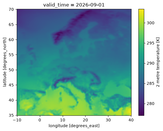
Now define the geographic average by weighting the latitude / longitude grid points by the cosine of the latitude.
[12]:
import numpy as np

lat_lon_weight = np.cos(np.deg2rad(aoi_temperature.latitude))

aoi_mean_temperature = aoi_temperature.weighted(lat_lon_weight).mean(
    ["latitude", "longitude"]
)
Until now we didn’t download any data (except one month for the plot above), the .compute() performs both the download and the computation step.
The following cell may run for a few minutes, depending on the speed of your network.
[13]:
%%time

aoi_mean_temperature_computed = aoi_mean_temperature.compute()
CPU times: user 1.74 s, sys: 506 ms, total: 2.25 s
Wall time: 23.3 s
Finally we compute the temperature change as the difference from the 1981-2010 average of the same calendar month, and plot the resulting time series:
[14]:
reference_period = aoi_mean_temperature_computed.sel(valid_time=slice("1981", "2010"))
climatology = reference_period.groupby("valid_time.month").mean()

temperature_change = (
    aoi_mean_temperature_computed.groupby("valid_time.month") - climatology
)
temperature_change.attrs["long_name"] = "temperature change since 1981-2010"
temperature_change.attrs["units"] = "°C"

_ = temperature_change.plot()
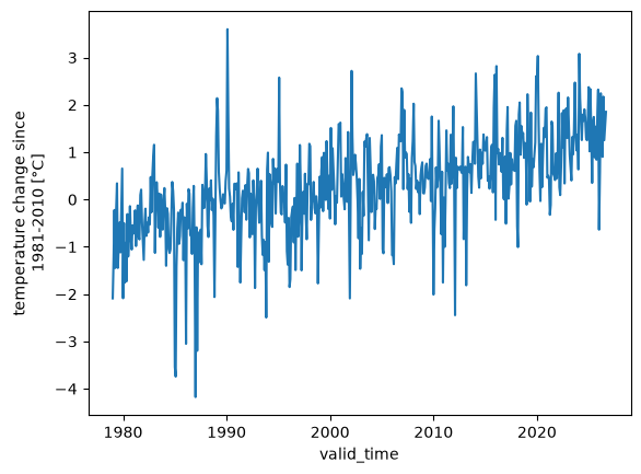
Again! Be careful, do not try to download an entire dataset, chances are that you will exceed your quota well before you come even close! Instead, we show how to access and work with large datasets in our tutorials.