How to work with ERA5 single levels on Earth Data Hub: climatological analysis of temperature in Germany#

Earth Data Hub (EDH) offers an innovative and super-efficient way to access earth related data. This notebook will provide you guidance on how to access and use the ERA5 single levels dataset.

Goal of this tutorial#

The first goal of this tutorial is to compute the 2 metre temperature anomaly for the month of October 2023, in the Germany area, against the 1991-2020 reference period.

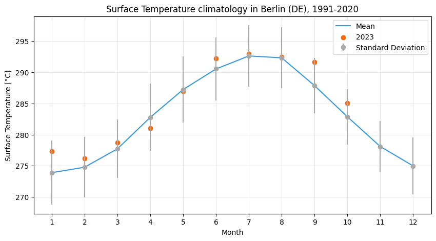
The second goal of this tutorial is to compute the 2 metre temperature climatology (monthly means and standard deviations) in Berlin for the same reference period and compare it with the monthly averages of 2023.

What you will learn:#

how to access the dataset
select and reduce the data
plot the results

To access datasets on Earth Data Hub you need to instruct your tools (xarray, Zarr, etc.) to use EDH personal access token when downloading the data.

To obtain a personal access token you first need to register to the Destination Earth platform. Then you can go to Earth Data Hub account settings where you can find your default personal access token or create others. After retrieving your personal access token, please cut and paste it below: ⤵

[ ]:

PAT = "your_EHD_personal_access_token"

#e.g. PAT="edh_pat_44bbb7e9192a4c6bb47ddf07d07564eee5d17de8dfc48f7118f88e3bc4a4157f8fe2403f5aa0a2d53441b6922ea9a33a"

We will use it later when accessing the dataset.

Working with EDH data#

Datasets on Earth Data Hub are often very large and remotely hosted. Typical use imply a selection of the data followed by one or more reduction steps to be performed in a local or distributed Dask environment.

The structure of a workflow that uses EDH data typically looks like this:

Data access
Data selection
Data reduction (optional)
Data download
Further operations and visualisation

Xarray and Dask work together following a lazy principle. This means that when you access and manipulate a Zarr store the data is in not immediately downloaded and loaded in memory. Instead, Dask constructs a task graph that represents the operations to be performed. A smart user will first reduce the amount of data that needs to be downloaded and explicitly call compute() on it. Once the compute() operation is complete the data is loaded into memory and available for subsequent fast processing.

1. Data access#

To access the data, only the dataset metadata must be downloaded. Xarray does this automatically when you access a Zarr dataset:

[ ]:

import xarray as xr
xr.set_options(keep_attrs=True)


ds = xr.open_dataset(
    f"https://edh:{PAT}@data.earthdatahub.destine.eu/era5/reanalysis-era5-single-levels-v0.zarr",
    chunks={},
    engine="zarr",
)
ds

<xarray.Dataset> Size: 405TB
Dimensions:     (valid_time: 756768, latitude: 721, longitude: 1440)
Coordinates:
  * valid_time  (valid_time) datetime64[ns] 6MB 1940-01-01 ... 2026-04-30T23:...
  * latitude    (latitude) float64 6kB 90.0 89.75 89.5 ... -89.5 -89.75 -90.0
  * longitude   (longitude) float64 12kB 0.0 0.25 0.5 0.75 ... 359.2 359.5 359.8
    number      int64 8B ...
    surface     float64 8B ...
Data variables: (12/129)
    alnid       (valid_time, latitude, longitude) float32 3TB dask.array<chunksize=(4320, 64, 64), meta=np.ndarray>
    alnip       (valid_time, latitude, longitude) float32 3TB dask.array<chunksize=(4320, 64, 64), meta=np.ndarray>
    aluvd       (valid_time, latitude, longitude) float32 3TB dask.array<chunksize=(4320, 64, 64), meta=np.ndarray>
    aluvp       (valid_time, latitude, longitude) float32 3TB dask.array<chunksize=(4320, 64, 64), meta=np.ndarray>
    anor        (valid_time, latitude, longitude) float32 3TB dask.array<chunksize=(4320, 64, 64), meta=np.ndarray>
    asn         (valid_time, latitude, longitude) float32 3TB dask.array<chunksize=(4320, 64, 64), meta=np.ndarray>
    ...          ...
    viiwn       (valid_time, latitude, longitude) float32 3TB dask.array<chunksize=(4320, 64, 64), meta=np.ndarray>
    vilwd       (valid_time, latitude, longitude) float32 3TB dask.array<chunksize=(4320, 64, 64), meta=np.ndarray>
    vilwe       (valid_time, latitude, longitude) float32 3TB dask.array<chunksize=(4320, 64, 64), meta=np.ndarray>
    vilwn       (valid_time, latitude, longitude) float32 3TB dask.array<chunksize=(4320, 64, 64), meta=np.ndarray>
    z           (valid_time, latitude, longitude) float32 3TB dask.array<chunksize=(4320, 64, 64), meta=np.ndarray>
    zust        (valid_time, latitude, longitude) float32 3TB dask.array<chunksize=(4320, 64, 64), meta=np.ndarray>
Attributes:
    Conventions:             CF-1.7
    GRIB_centre:             ecmf
    GRIB_centreDescription:  European Centre for Medium-Range Weather Forecasts
    GRIB_edition:            1
    GRIB_subCentre:          0
    history:                 2025-12-04T16:25 GRIB to CDM+CF via cfgrib-0.9.1...
    institution:             European Centre for Medium-Range Weather Forecasts

⚠ At this point, no data has been downloaded yet, nor loaded in memory.

2. Data selection#

Average 2 metre temperature in Germany, October 2023#

First, we perform a geographical selection corresponding to the Germany area. This greatly reduces the amount of data that will be downloaded from EDH. Also, we convert the temperature to °C.

[ ]:

t2m = ds.t2m
t2m_germany= t2m.sel(**{"latitude": slice(55, 47), "longitude": slice(5, 16)})
t2m_germany

<xarray.DataArray 't2m' (valid_time: 756768, latitude: 33, longitude: 45)> Size: 4GB
dask.array<getitem, shape=(756768, 33, 45), dtype=float32, chunksize=(4320, 33, 44), chunktype=numpy.ndarray>
Coordinates:
  * valid_time  (valid_time) datetime64[ns] 6MB 1940-01-01 ... 2026-04-30T23:...
  * latitude    (latitude) float64 264B 55.0 54.75 54.5 ... 47.5 47.25 47.0
  * longitude   (longitude) float64 360B 5.0 5.25 5.5 5.75 ... 15.5 15.75 16.0
    number      int64 8B ...
    surface     float64 8B ...
Attributes: (12/31)
    GRIB_NV:                                  0
    GRIB_Nx:                                  1440
    GRIB_Ny:                                  721
    GRIB_cfName:                              unknown
    GRIB_cfVarName:                           t2m
    GRIB_dataType:                            an
    ...                                       ...
    GRIB_typeOfLevel:                         surface
    GRIB_units:                               K
    GRIB_uvRelativeToGrid:                    0
    long_name:                                2 metre temperature
    standard_name:                            unknown
    units:                                    K

Second, we further select the October 2023 month. This is, again, a lazy operation:

[ ]:

t2m_germany_october_2023 = t2m_germany.sel(valid_time="2023-10")
t2m_germany_october_2023

<xarray.DataArray 't2m' (valid_time: 744, latitude: 33, longitude: 45)> Size: 4MB
dask.array<getitem, shape=(744, 33, 45), dtype=float32, chunksize=(480, 33, 44), chunktype=numpy.ndarray>
Coordinates:
  * valid_time  (valid_time) datetime64[ns] 6kB 2023-10-01 ... 2023-10-31T23:...
  * latitude    (latitude) float64 264B 55.0 54.75 54.5 ... 47.5 47.25 47.0
  * longitude   (longitude) float64 360B 5.0 5.25 5.5 5.75 ... 15.5 15.75 16.0
    number      int64 8B ...
    surface     float64 8B ...
Attributes: (12/31)
    GRIB_NV:                                  0
    GRIB_Nx:                                  1440
    GRIB_Ny:                                  721
    GRIB_cfName:                              unknown
    GRIB_cfVarName:                           t2m
    GRIB_dataType:                            an
    ...                                       ...
    GRIB_typeOfLevel:                         surface
    GRIB_units:                               K
    GRIB_uvRelativeToGrid:                    0
    long_name:                                2 metre temperature
    standard_name:                            unknown
    units:                                    K

3. Data download#

Due to the chunked structure of the DataArray, xarray will must download every chunk that includes a portion of the selected data.

To estimate the size of the download, we can use the costing.py module. This estimate must be done before we apply any reduction operation.

[ ]:

import costing

costing.estimate_download_size(t2m_germany_october_2023)

Estimated download size: 0.053 GiB (54.0 MiB)

At this point the selection is small enough to call compute() on it. This will trigger the download of data from EDH and load it in memory.

Remember to assign the return of the compute() function to a new variable, so that the data is kept in memory.

We can measure the time it takes:

[ ]:

%%time

t2m_germany_october_2023_computed = t2m_germany_october_2023.compute()

CPU times: user 1.21 s, sys: 617 ms, total: 1.83 s
Wall time: 1.82 s

The data was very small, this didn’t take long!

5. Visualisation#

Finally, we can plot the october 2023 monthly mean on a map:

[ ]:

import display
import matplotlib.pyplot as plt
from cartopy import crs

[ ]:

t2m_germany_october_2023_monthly_mean_degC = t2m_germany_october_2023_monthly_mean - 273.15
t2m_germany_october_2023_monthly_mean_degC.attrs["units"] = "°C"

display.map(
    t2m_germany_october_2023_monthly_mean_degC,
    projection=crs.Miller(),
    vmax=None,
    cmap="YlOrRd",
    title="Mean Surface Temperature, Oct 2023"
);

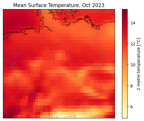
../../_images/notebooks_insula-code-lab_tutorial-era5-single-levels-climatological-analysis-of-temperature-in-germany_24_0.png

2 metre temperature anomaly in Germany, October 2023#

We want to compute the 2 metre temperature anomaly for the month of October 2023 against the 1991-2020 reference period, once again in Germany. The same considerations done before apply here.

We fist select the relevant months in the reference period:

[ ]:

t2m_germany_octobers_1991_2020 = t2m_germany.sel(valid_time=t2m_germany["valid_time.month"] == 10).sel(valid_time=slice("1991", "2020"))
t2m_germany_octobers_1991_2020

<xarray.DataArray 't2m' (valid_time: 22320, latitude: 33, longitude: 45)> Size: 133MB
dask.array<getitem, shape=(22320, 33, 45), dtype=float32, chunksize=(4299, 33, 44), chunktype=numpy.ndarray>
Coordinates:
  * valid_time  (valid_time) datetime64[ns] 179kB 1991-10-01 ... 2020-10-31T2...
  * latitude    (latitude) float64 264B 55.0 54.75 54.5 ... 47.5 47.25 47.0
  * longitude   (longitude) float64 360B 5.0 5.25 5.5 5.75 ... 15.5 15.75 16.0
    number      int64 8B ...
    surface     float64 8B ...
Attributes: (12/31)
    GRIB_NV:                                  0
    GRIB_Nx:                                  1440
    GRIB_Ny:                                  721
    GRIB_cfName:                              unknown
    GRIB_cfVarName:                           t2m
    GRIB_dataType:                            an
    ...                                       ...
    GRIB_typeOfLevel:                         surface
    GRIB_units:                               K
    GRIB_uvRelativeToGrid:                    0
    long_name:                                2 metre temperature
    standard_name:                            unknown
    units:                                    K

[ ]:

import costing

costing.estimate_download_size(t2m_germany_octobers_1991_2020)

Estimated download size: 0.185 GiB (189.0 MiB)

This is small enough to be computed in reasonable time:

[ ]:

%%time

t2m_germany_octobers_1991_2020_computed = t2m_germany_octobers_1991_2020.compute()

CPU times: user 17.3 s, sys: 10.3 s, total: 27.6 s
Wall time: 19.2 s

Now that the data is loaded in memory we can easily compute the 1991-2020 octobers mean:

[ ]:

t2m_germany_octobers_1991_2020_mean = t2m_germany_octobers_1991_2020_computed.mean(dim="valid_time")

And finally the anomaly:

[ ]:

anomaly = t2m_germany_october_2023_monthly_mean - t2m_germany_octobers_1991_2020_mean
anomaly

We can plot the anomaly on a map:

[ ]:

anomaly.attrs["units"] = "°C"

display.map(
    anomaly,
    vmax=None,
    projection=crs.Miller(),
    cmap="YlOrRd",
    title="Mean Surface Temperature anomaly (ref 1991-2020), Oct 2013"
);

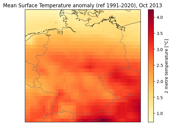
../../_images/notebooks_insula-code-lab_tutorial-era5-single-levels-climatological-analysis-of-temperature-in-germany_35_0.png

2 metre temperature climatology (1991-2020) in Berlin vs 2023 monthly mean#

The power of Earth Data Hub is better shown when working with timeseries. We will now show how fast is to compute the 2 metre temperature climatology (monthly mean and standard deviation) in Berlin, over the reference period 1991-2020, and compare it with the 2023 monthly means.

With legacy data distributon systems you would need to download the entire world temperature for the reference time period, extract the Berlin data and do your calculations. Alternatively the data provider might do a crop and merge operation for you, but chances are that this is very slow (internally the data provider still accesses the entire world temperature, you just don’t see it!). Thanks to Earth Data Hub this is not needed anymore. You only need to download the relevant chunks.

Here, we select the closest data to Berlin:

[ ]:

t2m_Berlin = t2m.sel(**{"latitude": 52.5, "longitude": 13.4}, method="nearest")
t2m_Berlin

<xarray.DataArray 't2m' (valid_time: 756768)> Size: 3MB
dask.array<getitem, shape=(756768,), dtype=float32, chunksize=(4320,), chunktype=numpy.ndarray>
Coordinates:
  * valid_time  (valid_time) datetime64[ns] 6MB 1940-01-01 ... 2026-04-30T23:...
    latitude    float64 8B 52.5
    longitude   float64 8B 13.5
    number      int64 8B ...
    surface     float64 8B ...
Attributes: (12/31)
    GRIB_NV:                                  0
    GRIB_Nx:                                  1440
    GRIB_Ny:                                  721
    GRIB_cfName:                              unknown
    GRIB_cfVarName:                           t2m
    GRIB_dataType:                            an
    ...                                       ...
    GRIB_typeOfLevel:                         surface
    GRIB_units:                               K
    GRIB_uvRelativeToGrid:                    0
    long_name:                                2 metre temperature
    standard_name:                            unknown
    units:                                    K

[ ]:

costing.estimate_download_size(t2m_Berlin)

Estimated download size: 2.32 GiB (2,376.0 MiB)

This is already small enough to be computed:

[ ]:

%%time

t2m_Berlin_computed = t2m_Berlin.compute()

CPU times: user 34.7 s, sys: 17.8 s, total: 52.4 s
Wall time: 49 s

Now that the data is loaded in memory we can easily compute the climatology for the reference period 1991-2020:

[ ]:

t2m_Berlin_climatology_mean = t2m_Berlin_computed.sel(valid_time=slice("1991", "2020")).groupby("valid_time.month").mean(dim="valid_time")
t2m_Berlin_climatology_std = t2m_Berlin_computed.sel(valid_time=slice("1991", "2020")).groupby("valid_time.month").std(dim="valid_time")

We also compute the monthly means for the year 2023:

[ ]:

t2m_Berlin_2023_monthly_means = t2m_Berlin_computed.sel(valid_time="2023").resample(valid_time="1ME").mean(dim="valid_time")
t2m_Berlin_2023_monthly_means

We can finally plot the climatology in Berlin for the 1991-2020 reference period against the 2023 monthly means:

[ ]:

plt.figure(figsize=(10, 5))
t2m_Berlin_climatology_mean.plot(label="Mean", color="#3498db")
plt.errorbar(
    t2m_Berlin_climatology_mean.month,
    t2m_Berlin_climatology_mean,
    yerr=t2m_Berlin_climatology_std,
    fmt="o",
    label="Standard Deviation",
    color="#a9a9a9"
)
for month in range (1, 11):
    t2m_point = t2m_Berlin_2023_monthly_means.sel(valid_time=t2m_Berlin_2023_monthly_means["valid_time.month"]==month)
    label = None
    if month == 1:
        label = "2023"
    plt.scatter(month, t2m_point, color="#ff6600", label=label)
plt.title("Surface Temperature climatology in Berlin (DE), 1991-2020")
plt.xticks(t2m_Berlin_climatology_mean.month)
plt.xlabel("Month")
plt.ylabel("Surface Temperature [°C]")
plt.legend()
plt.grid(alpha=0.3)
plt.show()

../../_images/notebooks_insula-code-lab_tutorial-era5-single-levels-climatological-analysis-of-temperature-in-germany_47_0.png