Multisource datasets integration: population weighted temperature from ERA5 and#

This notebook will provide you guidance on how to access and use the ERA5 single level dataset on Earth Data Hub, together with the Hybrid gridded demographic data for the world dataset worldwide demographic.

ERA5 single level data contains variables describing the global climate and weather for the past 8 decades. Data is available from 1940 onwards on a regular lat-lon grid of 0.25 degrees.

The Hybrid gridded demographic totals for the world contains the 1950-2020 demographic given as 5-year population bands at a 0.25 degree grid resolution.

Goal of this tutorial#

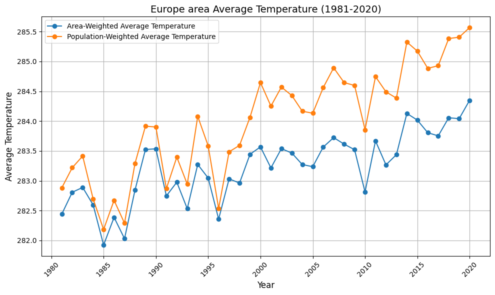
The goal of this tutorial is to visualize the area-averaged temperature in Europe as a function of time, and compare it with the population-averaged temperature.

What you will learn:#

how to access the data
select and reduce the data
use different datasets together
plot the results

To access datasets on Earth Data Hub (EDH) you need to instruct your tools (xarray, Zarr, etc.) to use EDH personal access token when downloading the data.

To obtain a personal access token you first need to register to the Destination Earth platform platform. Then you can go to Earth Data Hub account settings where you can find your default personal access token or create others. After retrieving your personal access token, please cut and paste it below: ⤵

[ ]:

PAT = "your_EHD_personal_access_token"

# e.g. PAT="edh_pat_44bbb7e9192a4c6bb47ddf07d07564eee5d17de8dfc48f7118f88e3bc4a4157f8fe2403f5aa0a2d53441b6922ea9a33a"

Working with EDH data#

Datasets on Earth Data Hub are often very large and remotely hosted. Typical use imply a selection of the data followed by one or more reduction steps to be performed in a local or distributed Dask environment.

The structure of a workflow that uses EDH data typically looks like this:

Data access
Data selection
Data reduction (optional)
Data download
Further operations and visualisation

Xarray and Dask work together following a lazy principle. This means that when you access and manipulate a Zarr store the data is in not immediately downloaded and loaded in memory. Instead, Dask constructs a task graph that represents the operations to be performed. A smart user will first reduce the amount of data that needs to be downloaded and explicitly call compute() on it. Once the compute() operation is complete the data is loaded into memory and available for subsequent fast processing.

1. Data access#

To access the data, only the dataset metadata must be downloaded. Xarray does this automatically when you access a Zarr dataset.

Preparing the population data#

[ ]:

import xarray as xr

world_population = xr.open_dataset(
    f"https://edh:{PAT}@data.earthdatahub.destine.eu/derived-GPWv4-Histsoc/demographics-hybrid-1950-2020-15-min-v0",
    chunks={},
    engine="zarr",
    storage_options={"client_kwargs": {"trust_env": True}},
)
world_population = world_population.demographic_totals
world_population

<xarray.DataArray 'demographic_totals' (latitude: 720, longitude: 1440,
                                        age_band_lower_bound: 14, year: 71)> Size: 4GB
dask.array<open_dataset-demographic_totals, shape=(720, 1440, 14, 71), dtype=float32, chunksize=(64, 64, 14, 71), chunktype=numpy.ndarray>
Coordinates:
  * latitude              (latitude) float64 6kB 90.0 89.75 ... -89.5 -89.75
  * longitude             (longitude) float64 12kB 0.0 0.25 0.5 ... 359.5 359.8
  * age_band_lower_bound  (age_band_lower_bound) int64 112B 0 5 10 ... 55 60 65
  * year                  (year) int64 568B 1950 1951 1952 ... 2018 2019 2020

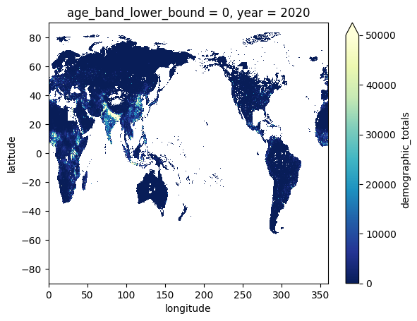
The longitude of the dataset is set from 0 to 360 degrees, which makes it uncomfortable to deal with data in the European area when using xarray:

[ ]:

world_population.sel(age_band_lower_bound=0, year=2020).plot(vmax=50_000, cmap="YlGnBu_r")

<matplotlib.collections.QuadMesh at 0x7f46a19ab7a0>

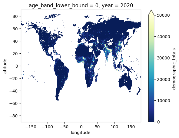
../../_images/notebooks_insula-code-lab_tutorial-population-weighted-temperature_8_1.png

We can roll the longitude to a -180 to 180 extent:

[ ]:

xr.set_options(keep_attrs=True)

world_population = world_population.assign_coords(longitude=(((world_population.longitude + 180) % 360) - 180))
world_population = world_population.roll(longitude=int(len(world_population.longitude) / 2), roll_coords=True)
world_population

<xarray.DataArray 'demographic_totals' (latitude: 720, longitude: 1440,
                                        age_band_lower_bound: 14, year: 71)> Size: 4GB
dask.array<rechunk-merge, shape=(720, 1440, 14, 71), dtype=float32, chunksize=(64, 64, 14, 71), chunktype=numpy.ndarray>
Coordinates:
  * latitude              (latitude) float64 6kB 90.0 89.75 ... -89.5 -89.75
  * longitude             (longitude) float64 12kB -180.0 -179.8 ... 179.5 179.8
  * age_band_lower_bound  (age_band_lower_bound) int64 112B 0 5 10 ... 55 60 65
  * year                  (year) int64 568B 1950 1951 1952 ... 2018 2019 2020

[ ]:

world_population.sel(age_band_lower_bound=0, year=2020).plot(vmax=50_000, cmap="YlGnBu_r")

<matplotlib.collections.QuadMesh at 0x7f46b1310e00>

../../_images/notebooks_insula-code-lab_tutorial-population-weighted-temperature_11_1.png

2. Data selection#

On the world data, we perform a geographical selection corresponding to continental Europe:

[ ]:

europe_population = world_population.sel(latitude=slice(71, 36), longitude=slice(-10,35))
europe_population

<xarray.DataArray 'demographic_totals' (latitude: 141, longitude: 181,
                                        age_band_lower_bound: 14, year: 71)> Size: 101MB
dask.array<getitem, shape=(141, 181, 14, 71), dtype=float32, chunksize=(64, 64, 14, 71), chunktype=numpy.ndarray>
Coordinates:
  * latitude              (latitude) float64 1kB 71.0 70.75 70.5 ... 36.25 36.0
  * longitude             (longitude) float64 1kB -10.0 -9.75 ... 34.75 35.0
  * age_band_lower_bound  (age_band_lower_bound) int64 112B 0 5 10 ... 55 60 65
  * year                  (year) int64 568B 1950 1951 1952 ... 2018 2019 2020

This is a relatively small dataset, we don’t need to worry too much about the download size.

3. Data reduction#

Next, we calculate the total population for each and every year. Notice that the data spans from 1950 to 2020.

[ ]:

europe_population_bands_total = europe_population.sum("age_band_lower_bound")
europe_population_bands_total

<xarray.DataArray 'demographic_totals' (latitude: 141, longitude: 181, year: 71)> Size: 7MB
dask.array<sum-aggregate, shape=(141, 181, 71), dtype=float32, chunksize=(64, 64, 71), chunktype=numpy.ndarray>
Coordinates:
  * latitude   (latitude) float64 1kB 71.0 70.75 70.5 70.25 ... 36.5 36.25 36.0
  * longitude  (longitude) float64 1kB -10.0 -9.75 -9.5 ... 34.5 34.75 35.0
  * year       (year) int64 568B 1950 1951 1952 1953 ... 2017 2018 2019 2020

xarray.DataArray

'demographic_totals'

latitude: 141
longitude: 181
year: 71

dask.array<chunksize=(52, 24, 71), meta=np.ndarray>

	Array	Chunk
Bytes	6.91 MiB	1.11 MiB
Shape	(141, 181, 71)	(64, 64, 71)
Dask graph	12 chunks in 12 graph layers
Data type	float32 numpy.ndarray

Coordinates: (3)

latitude

(latitude)

float64

71.0 70.75 70.5 ... 36.5 36.25 36.0

array([71.  , 70.75, 70.5 , 70.25, 70.  , 69.75, 69.5 , 69.25, 69.  , 68.75,
       68.5 , 68.25, 68.  , 67.75, 67.5 , 67.25, 67.  , 66.75, 66.5 , 66.25,
       66.  , 65.75, 65.5 , 65.25, 65.  , 64.75, 64.5 , 64.25, 64.  , 63.75,
       63.5 , 63.25, 63.  , 62.75, 62.5 , 62.25, 62.  , 61.75, 61.5 , 61.25,
       61.  , 60.75, 60.5 , 60.25, 60.  , 59.75, 59.5 , 59.25, 59.  , 58.75,
       58.5 , 58.25, 58.  , 57.75, 57.5 , 57.25, 57.  , 56.75, 56.5 , 56.25,
       56.  , 55.75, 55.5 , 55.25, 55.  , 54.75, 54.5 , 54.25, 54.  , 53.75,
       53.5 , 53.25, 53.  , 52.75, 52.5 , 52.25, 52.  , 51.75, 51.5 , 51.25,
       51.  , 50.75, 50.5 , 50.25, 50.  , 49.75, 49.5 , 49.25, 49.  , 48.75,
       48.5 , 48.25, 48.  , 47.75, 47.5 , 47.25, 47.  , 46.75, 46.5 , 46.25,
       46.  , 45.75, 45.5 , 45.25, 45.  , 44.75, 44.5 , 44.25, 44.  , 43.75,
       43.5 , 43.25, 43.  , 42.75, 42.5 , 42.25, 42.  , 41.75, 41.5 , 41.25,
       41.  , 40.75, 40.5 , 40.25, 40.  , 39.75, 39.5 , 39.25, 39.  , 38.75,
       38.5 , 38.25, 38.  , 37.75, 37.5 , 37.25, 37.  , 36.75, 36.5 , 36.25,
       36.  ])

longitude

(longitude)

float64

-10.0 -9.75 -9.5 ... 34.75 35.0

array([-10.  ,  -9.75,  -9.5 ,  -9.25,  -9.  ,  -8.75,  -8.5 ,  -8.25,  -8.  ,
        -7.75,  -7.5 ,  -7.25,  -7.  ,  -6.75,  -6.5 ,  -6.25,  -6.  ,  -5.75,
        -5.5 ,  -5.25,  -5.  ,  -4.75,  -4.5 ,  -4.25,  -4.  ,  -3.75,  -3.5 ,
        -3.25,  -3.  ,  -2.75,  -2.5 ,  -2.25,  -2.  ,  -1.75,  -1.5 ,  -1.25,
        -1.  ,  -0.75,  -0.5 ,  -0.25,   0.  ,   0.25,   0.5 ,   0.75,   1.  ,
         1.25,   1.5 ,   1.75,   2.  ,   2.25,   2.5 ,   2.75,   3.  ,   3.25,
         3.5 ,   3.75,   4.  ,   4.25,   4.5 ,   4.75,   5.  ,   5.25,   5.5 ,
         5.75,   6.  ,   6.25,   6.5 ,   6.75,   7.  ,   7.25,   7.5 ,   7.75,
         8.  ,   8.25,   8.5 ,   8.75,   9.  ,   9.25,   9.5 ,   9.75,  10.  ,
        10.25,  10.5 ,  10.75,  11.  ,  11.25,  11.5 ,  11.75,  12.  ,  12.25,
        12.5 ,  12.75,  13.  ,  13.25,  13.5 ,  13.75,  14.  ,  14.25,  14.5 ,
        14.75,  15.  ,  15.25,  15.5 ,  15.75,  16.  ,  16.25,  16.5 ,  16.75,
        17.  ,  17.25,  17.5 ,  17.75,  18.  ,  18.25,  18.5 ,  18.75,  19.  ,
        19.25,  19.5 ,  19.75,  20.  ,  20.25,  20.5 ,  20.75,  21.  ,  21.25,
        21.5 ,  21.75,  22.  ,  22.25,  22.5 ,  22.75,  23.  ,  23.25,  23.5 ,
        23.75,  24.  ,  24.25,  24.5 ,  24.75,  25.  ,  25.25,  25.5 ,  25.75,
        26.  ,  26.25,  26.5 ,  26.75,  27.  ,  27.25,  27.5 ,  27.75,  28.  ,
        28.25,  28.5 ,  28.75,  29.  ,  29.25,  29.5 ,  29.75,  30.  ,  30.25,
        30.5 ,  30.75,  31.  ,  31.25,  31.5 ,  31.75,  32.  ,  32.25,  32.5 ,
        32.75,  33.  ,  33.25,  33.5 ,  33.75,  34.  ,  34.25,  34.5 ,  34.75,
        35.  ])

year

(year)

int64

1950 1951 1952 ... 2018 2019 2020

array([1950, 1951, 1952, 1953, 1954, 1955, 1956, 1957, 1958, 1959, 1960, 1961,
       1962, 1963, 1964, 1965, 1966, 1967, 1968, 1969, 1970, 1971, 1972, 1973,
       1974, 1975, 1976, 1977, 1978, 1979, 1980, 1981, 1982, 1983, 1984, 1985,
       1986, 1987, 1988, 1989, 1990, 1991, 1992, 1993, 1994, 1995, 1996, 1997,
       1998, 1999, 2000, 2001, 2002, 2003, 2004, 2005, 2006, 2007, 2008, 2009,
       2010, 2011, 2012, 2013, 2014, 2015, 2016, 2017, 2018, 2019, 2020])

4. Data download#

This is the phase where we explicitly trigger the download of the data. To do so we will call compute() on the European total population. The result will be small enough to easily fit into memory. Remember to assign the return of the compute() function to a new variable, so that the data is kept in memory.

We can measure the time it takes:

[ ]:

%%time

europe_population_bands_total_computed = europe_population_bands_total.compute()

CPU times: user 881 ms, sys: 163 ms, total: 1.04 s
Wall time: 2.44 s

Preparing ERA5-single levels data#

We will now follow the same logic to load ERA5 single levels data.

[ ]:

era5_single_levels = xr.open_dataset(
    f"https://edh:{PAT}@data.earthdatahub.destine.eu/era5/reanalysis-era5-single-levels-v0.zarr",
    chunks={},
    engine="zarr",
    storage_options={"client_kwargs": {"trust_env": True}},
)
era5_single_levels

<xarray.Dataset> Size: 405TB
Dimensions:     (valid_time: 756768, latitude: 721, longitude: 1440)
Coordinates:
  * valid_time  (valid_time) datetime64[ns] 6MB 1940-01-01 ... 2026-04-30T23:...
  * latitude    (latitude) float64 6kB 90.0 89.75 89.5 ... -89.5 -89.75 -90.0
  * longitude   (longitude) float64 12kB 0.0 0.25 0.5 0.75 ... 359.2 359.5 359.8
    number      int64 8B ...
    surface     float64 8B ...
Data variables: (12/129)
    alnid       (valid_time, latitude, longitude) float32 3TB dask.array<chunksize=(4320, 64, 64), meta=np.ndarray>
    alnip       (valid_time, latitude, longitude) float32 3TB dask.array<chunksize=(4320, 64, 64), meta=np.ndarray>
    aluvd       (valid_time, latitude, longitude) float32 3TB dask.array<chunksize=(4320, 64, 64), meta=np.ndarray>
    aluvp       (valid_time, latitude, longitude) float32 3TB dask.array<chunksize=(4320, 64, 64), meta=np.ndarray>
    anor        (valid_time, latitude, longitude) float32 3TB dask.array<chunksize=(4320, 64, 64), meta=np.ndarray>
    asn         (valid_time, latitude, longitude) float32 3TB dask.array<chunksize=(4320, 64, 64), meta=np.ndarray>
    ...          ...
    viiwn       (valid_time, latitude, longitude) float32 3TB dask.array<chunksize=(4320, 64, 64), meta=np.ndarray>
    vilwd       (valid_time, latitude, longitude) float32 3TB dask.array<chunksize=(4320, 64, 64), meta=np.ndarray>
    vilwe       (valid_time, latitude, longitude) float32 3TB dask.array<chunksize=(4320, 64, 64), meta=np.ndarray>
    vilwn       (valid_time, latitude, longitude) float32 3TB dask.array<chunksize=(4320, 64, 64), meta=np.ndarray>
    z           (valid_time, latitude, longitude) float32 3TB dask.array<chunksize=(4320, 64, 64), meta=np.ndarray>
    zust        (valid_time, latitude, longitude) float32 3TB dask.array<chunksize=(4320, 64, 64), meta=np.ndarray>
Attributes:
    Conventions:             CF-1.7
    GRIB_centre:             ecmf
    GRIB_centreDescription:  European Centre for Medium-Range Weather Forecasts
    GRIB_edition:            1
    GRIB_subCentre:          0
    history:                 2025-12-04T16:25 GRIB to CDM+CF via cfgrib-0.9.1...
    institution:             European Centre for Medium-Range Weather Forecasts

From the dataset we extract the 2 metre temperature:

[ ]:

t2m = era5_single_levels.t2m

We perform the same coordinate rolling as we did before:

[ ]:

t2m = t2m.assign_coords(longitude=(((t2m.longitude + 180) % 360) - 180))
t2m = t2m.roll(longitude=int(len(t2m.longitude) / 2), roll_coords=True)
t2m

<xarray.DataArray 't2m' (valid_time: 756768, latitude: 721, longitude: 1440)> Size: 3TB
dask.array<rechunk-merge, shape=(756768, 721, 1440), dtype=float32, chunksize=(4320, 64, 64), chunktype=numpy.ndarray>
Coordinates:
  * valid_time  (valid_time) datetime64[ns] 6MB 1940-01-01 ... 2026-04-30T23:...
  * latitude    (latitude) float64 6kB 90.0 89.75 89.5 ... -89.5 -89.75 -90.0
  * longitude   (longitude) float64 12kB -180.0 -179.8 -179.5 ... 179.5 179.8
    number      int64 8B ...
    surface     float64 8B ...
Attributes: (12/31)
    GRIB_NV:                                  0
    GRIB_Nx:                                  1440
    GRIB_Ny:                                  721
    GRIB_cfName:                              unknown
    GRIB_cfVarName:                           t2m
    GRIB_dataType:                            an
    ...                                       ...
    GRIB_typeOfLevel:                         surface
    GRIB_units:                               K
    GRIB_uvRelativeToGrid:                    0
    long_name:                                2 metre temperature
    standard_name:                            unknown
    units:                                    K

Also, we perform a geographical selection corresponding to continental Europe and a temporal selection of the years between 1981 and 2020.

[ ]:

t2m_europe = t2m.sel(latitude=slice(71, 36), longitude=slice(-10,35))
t2m_europe_1981_2020 = t2m_europe.sel(valid_time=slice("1981", "2020"))
t2m_europe_1981_2020

<xarray.DataArray 't2m' (valid_time: 350640, latitude: 141, longitude: 181)> Size: 36GB
dask.array<getitem, shape=(350640, 141, 181), dtype=float32, chunksize=(4320, 64, 64), chunktype=numpy.ndarray>
Coordinates:
  * valid_time  (valid_time) datetime64[ns] 3MB 1981-01-01 ... 2020-12-31T23:...
  * latitude    (latitude) float64 1kB 71.0 70.75 70.5 70.25 ... 36.5 36.25 36.0
  * longitude   (longitude) float64 1kB -10.0 -9.75 -9.5 ... 34.5 34.75 35.0
    number      int64 8B ...
    surface     float64 8B ...
Attributes: (12/31)
    GRIB_NV:                                  0
    GRIB_Nx:                                  1440
    GRIB_Ny:                                  721
    GRIB_cfName:                              unknown
    GRIB_cfVarName:                           t2m
    GRIB_dataType:                            an
    ...                                       ...
    GRIB_typeOfLevel:                         surface
    GRIB_units:                               K
    GRIB_uvRelativeToGrid:                    0
    long_name:                                2 metre temperature
    standard_name:                            unknown
    units:                                    K

The ERA5 single levels dataset is way bigger than the population one. When we access a sample of the 2 metre temperature, xarray must download every chunk that includes a portion of the selected data.

To estimate the size of the download, we can use the costing.py module. This estimate must be done before we apply any reduction operation.

[ ]:

import costing

costing.estimate_download_size(t2m_europe_1981_2020)

Estimated download size: 12.973 GiB (13,284.0 MiB)

This amount of data could be easily downloaded from Earth Data Hub, thanks to data compression. However, the result of the compute() wouldn’t fit into memory. We thus perform a reduction operation before triggering the download and computation, which greatly reduces the size of the result that will be kept in memory.

We compute the annual average of the 2 metre temperature:

[ ]:

t2m_europe_yearly_mean = t2m_europe_1981_2020.resample(valid_time="YS").mean()
t2m_europe_yearly_mean

<xarray.DataArray 't2m' (valid_time: 40, latitude: 141, longitude: 181)> Size: 4MB
dask.array<transpose, shape=(40, 141, 181), dtype=float32, chunksize=(1, 64, 64), chunktype=numpy.ndarray>
Coordinates:
  * valid_time  (valid_time) datetime64[ns] 320B 1981-01-01 ... 2020-01-01
  * latitude    (latitude) float64 1kB 71.0 70.75 70.5 70.25 ... 36.5 36.25 36.0
  * longitude   (longitude) float64 1kB -10.0 -9.75 -9.5 ... 34.5 34.75 35.0
    number      int64 8B ...
    surface     float64 8B ...
Attributes: (12/31)
    GRIB_NV:                                  0
    GRIB_Nx:                                  1440
    GRIB_Ny:                                  721
    GRIB_cfName:                              unknown
    GRIB_cfVarName:                           t2m
    GRIB_dataType:                            an
    ...                                       ...
    GRIB_typeOfLevel:                         surface
    GRIB_units:                               K
    GRIB_uvRelativeToGrid:                    0
    long_name:                                2 metre temperature
    standard_name:                            unknown
    units:                                    K

At this point, the resulting dataset small enough to call compute() on it. Remember to assign the return of the compute() function to a new variable, so that the data is kept in memory.

We can measure the time it takes:

[ ]:

%%time

t2m_europe_yearly_mean_computed = t2m_europe_yearly_mean.compute()

CPU times: user 11min 7s, sys: 3min 18s, total: 14min 26s
Wall time: 14min 40s

### Area-weighted 2 metre temperature vs population-weighted 2 metre temperature

To compute the area-weighted 2 metre temperature trend in Europe, we need to spatially average the temperature data using the areas of the latitude-longitude grid cells as weights:

[ ]:

import numpy as np

weights = np.cos(np.deg2rad(t2m_europe_yearly_mean_computed.latitude))
weights.name = "weights"

t2m_europe_yearly_mean_area_weighted = t2m_europe_yearly_mean_computed.weighted(weights).mean(("longitude", "latitude"))
t2m_europe_yearly_mean_area_weighted

<xarray.DataArray 't2m' (valid_time: 40)> Size: 320B
array([282.44060173, 282.80726744, 282.88833763, 282.59481572,
       281.92272722, 282.38664733, 282.02955936, 282.84208603,
       283.52346136, 283.53606642, 282.746041  , 282.97611395,
       282.53185087, 283.27298412, 283.04627173, 282.35752562,
       283.0313843 , 282.96213073, 283.44426336, 283.56753882,
       283.21514751, 283.53828153, 283.4645456 , 283.27169292,
       283.23578931, 283.56501609, 283.72337254, 283.61448899,
       283.52041778, 282.81172874, 283.66797716, 283.26656075,
       283.43727423, 284.12849353, 284.01713386, 283.80555228,
       283.7526294 , 284.05611564, 284.0403951 , 284.34887736])
Coordinates:
  * valid_time  (valid_time) datetime64[ns] 320B 1981-01-01 ... 2020-01-01
    number      int64 8B 0
    surface     float64 8B 0.0
Attributes: (12/31)
    GRIB_NV:                                  0
    GRIB_Nx:                                  1440
    GRIB_Ny:                                  721
    GRIB_cfName:                              unknown
    GRIB_cfVarName:                           t2m
    GRIB_dataType:                            an
    ...                                       ...
    GRIB_typeOfLevel:                         surface
    GRIB_units:                               K
    GRIB_uvRelativeToGrid:                    0
    long_name:                                2 metre temperature
    standard_name:                            unknown
    units:                                    K

xarray.DataArray

't2m'

valid_time: 40

282.4 282.8 282.9 282.6 281.9 282.4 ... 283.8 283.8 284.1 284.0 284.3

array([282.44060173, 282.80726744, 282.88833763, 282.59481572,
       281.92272722, 282.38664733, 282.02955936, 282.84208603,
       283.52346136, 283.53606642, 282.746041  , 282.97611395,
       282.53185087, 283.27298412, 283.04627173, 282.35752562,
       283.0313843 , 282.96213073, 283.44426336, 283.56753882,
       283.21514751, 283.53828153, 283.4645456 , 283.27169292,
       283.23578931, 283.56501609, 283.72337254, 283.61448899,
       283.52041778, 282.81172874, 283.66797716, 283.26656075,
       283.43727423, 284.12849353, 284.01713386, 283.80555228,
       283.7526294 , 284.05611564, 284.0403951 , 284.34887736])

Coordinates: (3)

valid_time

(valid_time)

datetime64[ns]

1981-01-01 ... 2020-01-01

array(['1981-01-01T00:00:00.000000000', '1982-01-01T00:00:00.000000000',
       '1983-01-01T00:00:00.000000000', '1984-01-01T00:00:00.000000000',
       '1985-01-01T00:00:00.000000000', '1986-01-01T00:00:00.000000000',
       '1987-01-01T00:00:00.000000000', '1988-01-01T00:00:00.000000000',
       '1989-01-01T00:00:00.000000000', '1990-01-01T00:00:00.000000000',
       '1991-01-01T00:00:00.000000000', '1992-01-01T00:00:00.000000000',
       '1993-01-01T00:00:00.000000000', '1994-01-01T00:00:00.000000000',
       '1995-01-01T00:00:00.000000000', '1996-01-01T00:00:00.000000000',
       '1997-01-01T00:00:00.000000000', '1998-01-01T00:00:00.000000000',
       '1999-01-01T00:00:00.000000000', '2000-01-01T00:00:00.000000000',
       '2001-01-01T00:00:00.000000000', '2002-01-01T00:00:00.000000000',
       '2003-01-01T00:00:00.000000000', '2004-01-01T00:00:00.000000000',
       '2005-01-01T00:00:00.000000000', '2006-01-01T00:00:00.000000000',
       '2007-01-01T00:00:00.000000000', '2008-01-01T00:00:00.000000000',
       '2009-01-01T00:00:00.000000000', '2010-01-01T00:00:00.000000000',
       '2011-01-01T00:00:00.000000000', '2012-01-01T00:00:00.000000000',
       '2013-01-01T00:00:00.000000000', '2014-01-01T00:00:00.000000000',
       '2015-01-01T00:00:00.000000000', '2016-01-01T00:00:00.000000000',
       '2017-01-01T00:00:00.000000000', '2018-01-01T00:00:00.000000000',
       '2019-01-01T00:00:00.000000000', '2020-01-01T00:00:00.000000000'],
      dtype='datetime64[ns]')

number
()
int64
0
long_name :
ensemble member numerical id
standard_name :
realization
units :
1
```
array(0)
```
surface
()
float64
0.0
long_name :
original GRIB coordinate for key: level(surface)
units :
1
```
array(0.)
```

Attributes: (31)
GRIB_NV :
0
GRIB_Nx :
1440
GRIB_Ny :
721
GRIB_cfName :
unknown
GRIB_cfVarName :
t2m
GRIB_dataType :
an
GRIB_gridDefinitionDescription :
Latitude/Longitude Grid
GRIB_gridType :
regular_ll
GRIB_iDirectionIncrementInDegrees :
0.25
GRIB_iScansNegatively :
0
GRIB_jDirectionIncrementInDegrees :
0.25
GRIB_jPointsAreConsecutive :
0
GRIB_jScansPositively :
0
GRIB_latitudeOfFirstGridPointInDegrees :
90.0
GRIB_latitudeOfLastGridPointInDegrees :
-90.0
GRIB_longitudeOfFirstGridPointInDegrees :
0.0
GRIB_longitudeOfLastGridPointInDegrees :
359.75
GRIB_missingValue :
3.4028234663852886e+38
GRIB_name :
2 metre temperature
GRIB_numberOfPoints :
1038240
GRIB_paramId :
167
GRIB_shortName :
2t
GRIB_stepType :
instant
GRIB_stepUnits :
1
GRIB_totalNumber :
0
GRIB_typeOfLevel :
surface
GRIB_units :
K
GRIB_uvRelativeToGrid :
0
long_name :
2 metre temperature
standard_name :
unknown
units :
K

To compute the population-weighted 2 metre temperature we will follow the same logic, but this time we will use the population data as weight. To make the population data and temperature data compatible we need to transform the valid_time coordinate of the temperature data to the yearcoordinate of the population data so that the two data array can be easily multiplied:

[ ]:

# shorten the names and replace the valid_time coordinate
temperature = t2m_europe_yearly_mean_computed.assign_coords({"year" : t2m_europe_yearly_mean_computed.valid_time.dt.year}).swap_dims({"valid_time": "year"}).drop_vars("valid_time")
population = europe_population_bands_total_computed

# compute the population weighted temperature
t2m_europe_yearly_mean_population_weighted = (temperature * population).sum(dim=["latitude", "longitude"]) / population.sum(dim=["latitude", "longitude"])

5. Visualisation#

Finally, we can compare the area-weighted temperature with the population-weighted temperature in the same graph. The first one is the average temperature experienced by the territory, while the second represents the average temperature experienced by people. Notice that the latter is higher than the first.

[ ]:

import matplotlib.pyplot as plt

plt.figure(figsize=(10, 6))
plt.plot(t2m_europe_yearly_mean_area_weighted.valid_time.dt.year, t2m_europe_yearly_mean_area_weighted, marker='o', label='Area-Weighted Average Temperature')
plt.plot(t2m_europe_yearly_mean_population_weighted.year, t2m_europe_yearly_mean_population_weighted, marker='o', label='Population-Weighted Average Temperature')
plt.legend()
plt.title("Europe area Average Temperature (1981-2020)", fontsize=14)
plt.xlabel("Year", fontsize=12)
plt.ylabel("Average Temperature", fontsize=12)
plt.grid(True)
plt.xticks(rotation=45)
plt.tight_layout()
plt.show()

../../_images/notebooks_insula-code-lab_tutorial-population-weighted-temperature_42_0.png